Analysis

Here each analysis script is described in a short summary and by its doc string.

CIRRUS-HL

CIRRUS-HL laboratory calibration comparison

Script: cirrus_hl_smart_compare_lab_calibs.py

CIRRUS-HL: Compare laboratory calibrations of SMART

For CIRRUS-HL two laboratory calibrations were done. Here the two calibrations are compared to each other.

The first lab calibration did not have the final optical fiber and inlet setting as were used during CIRRUS-HL. Thus, a difference between the after and before campaign calibration is to be expected. In addition to that, the optical fibers were unplugged after the campaign for the transport of SMART to Leipzig.

Each lab calibration is processed with smart_process_lab_calib.py to correct the files for the dark current. After that the calibration factors are calculated with analysis.smart_calib_lab_ASP06.py for ASP06 and analysis.smart_calib_lab_ASP07.py for ASP07.

• compare calibration factors

• compare Ulli measurements

Results

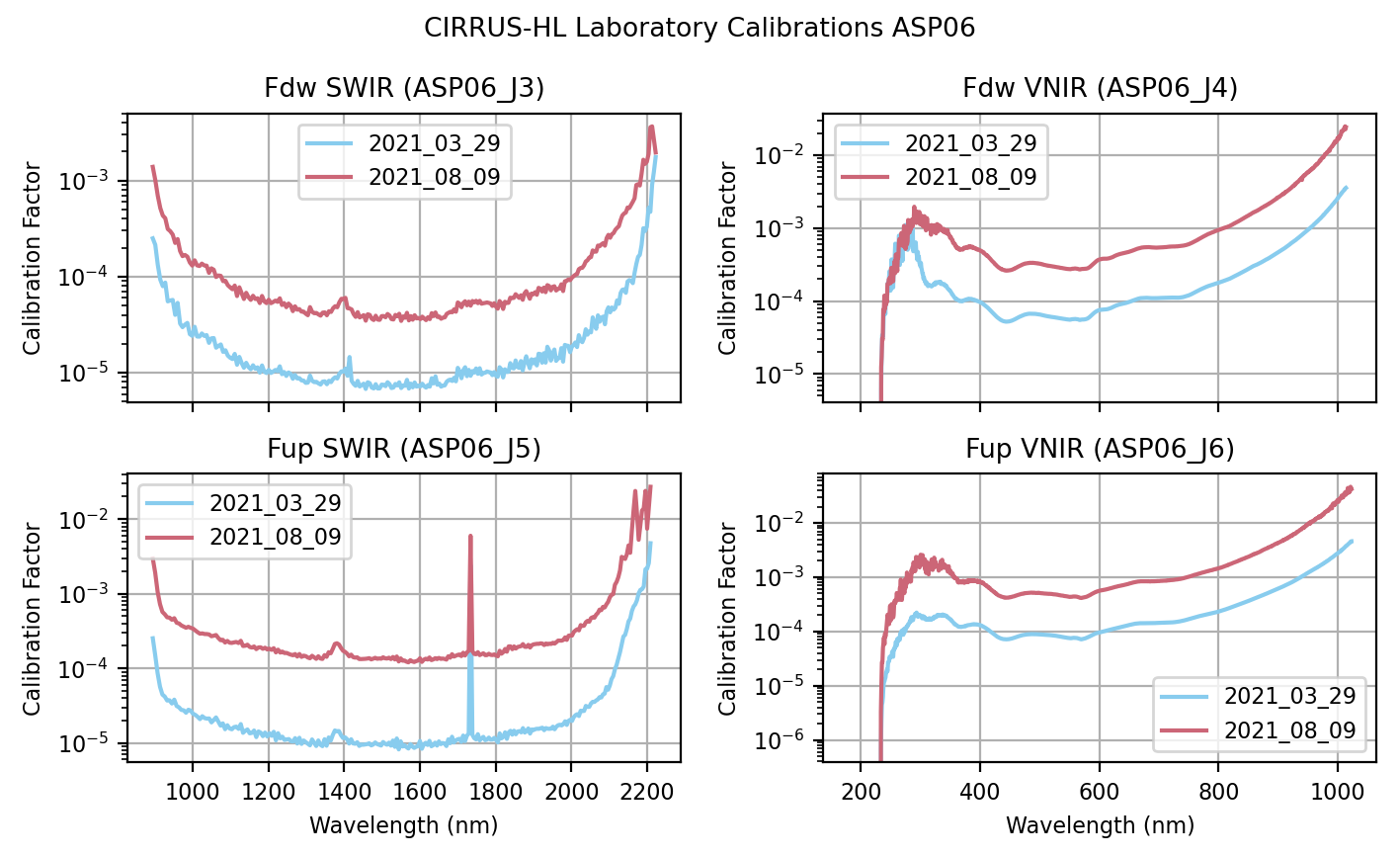
Fig. 44 Comparison of the lab calibration factors before and after CIRRUS-HL for the four channels on ASP06.

Comparing the calibration factors of ASP06 between the before and after calibration shows that the after calibration (red) has a higher magnitude. This is due to fewer counts being measured during the after calibration. A possible cause of this is that the cable used in the after calibration was longer and also showed signs of damage leading to a loss of photons on the way from the inlet to the spectrometer. To account for that a higher calibration factor is needed to calculate the given irradiance which did not change between the calibrations. The same result can be observed for the calibrations for ASP07.

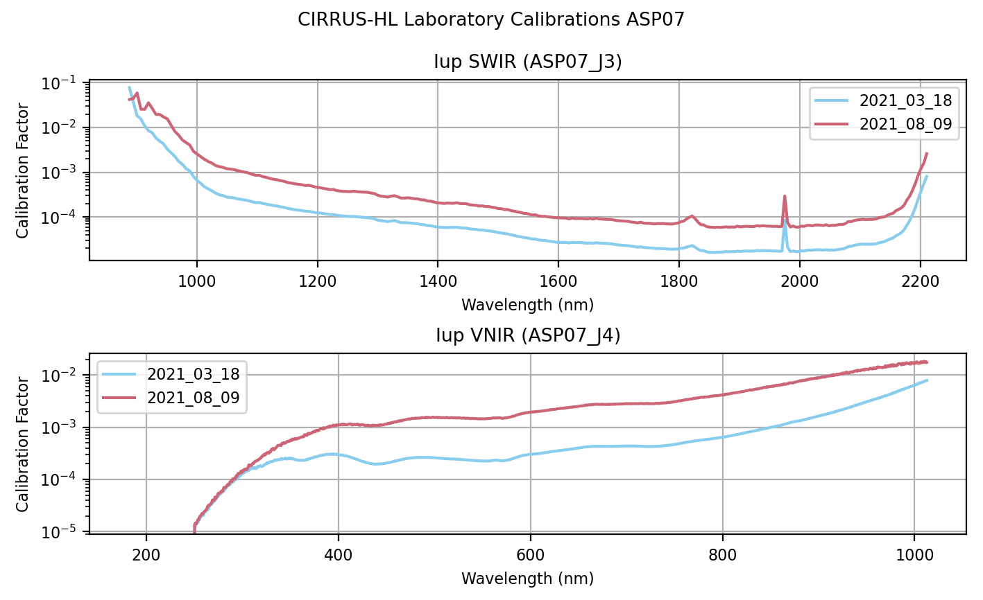
Fig. 45 Comparison of the lab calibration factors before and after CIRRUS-HL for the two channels on ASP07.

Ulli measurements

Taking a look at ASP06’s measurements of the Ulbricht sphere (Ulli) shows the same difference in magnitude between the calibrations when comparing the dark current corrected counts.

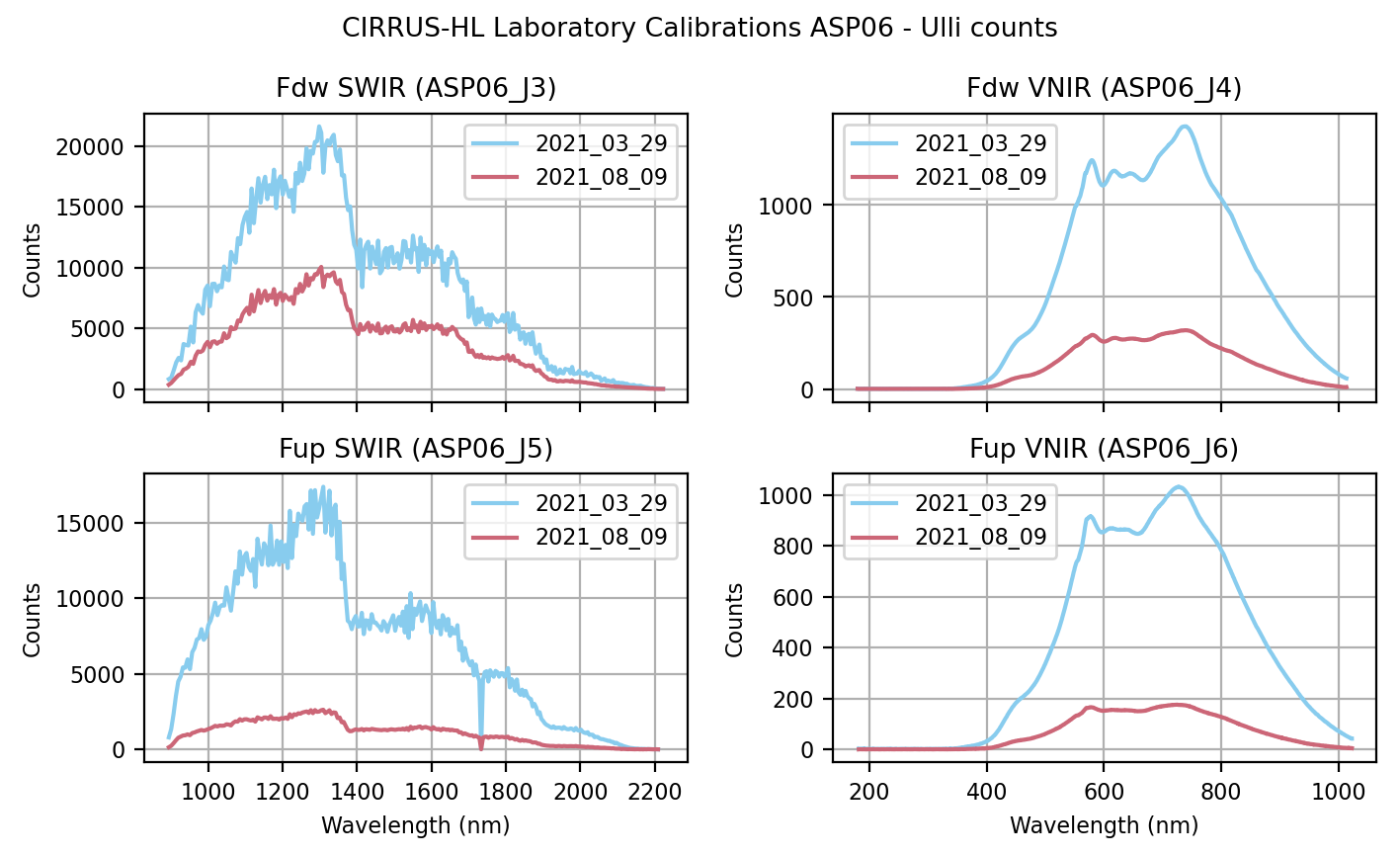
Fig. 46 Dark current corrected count measurements of the Ulli transfer sphere from ASP06.

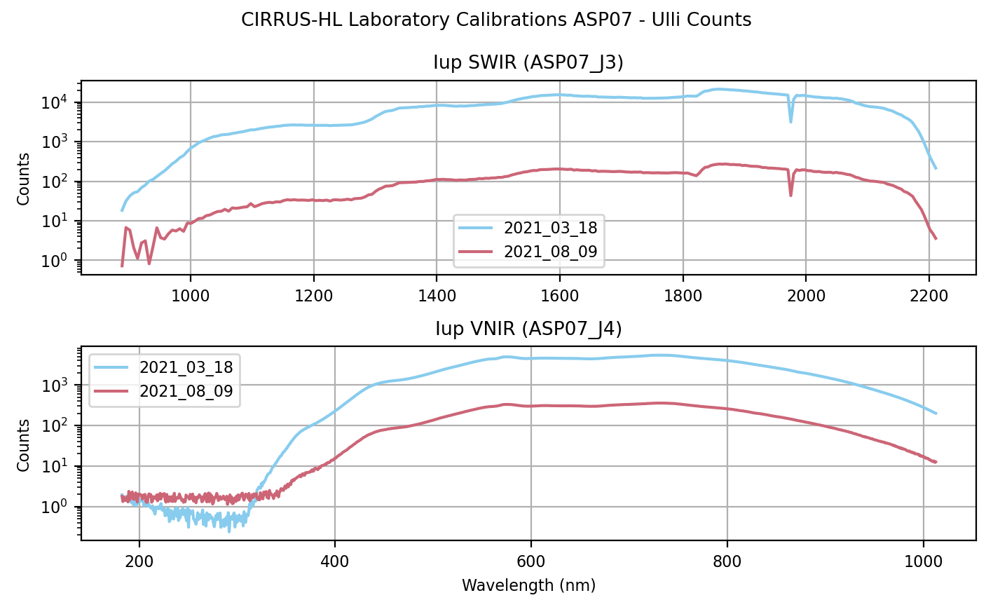
Fig. 47 Dark current corrected count measurements of the Ulli transfer sphere from ASP07.

It can clearly be seen that during the after calibration less photons reached the spectrometers. However, this should still result in the same irradiance as long as the Ulli sphere is run with the same power source and the same settings. Just like the output of the 1000W calibration lamp should not change between the calibration, so should the output of the Ulli sphere not change. Nonetheless, when looking at the calculated irradiance using the corresponding laboratory calibration factors clear differences can be observed for the downward measurements.

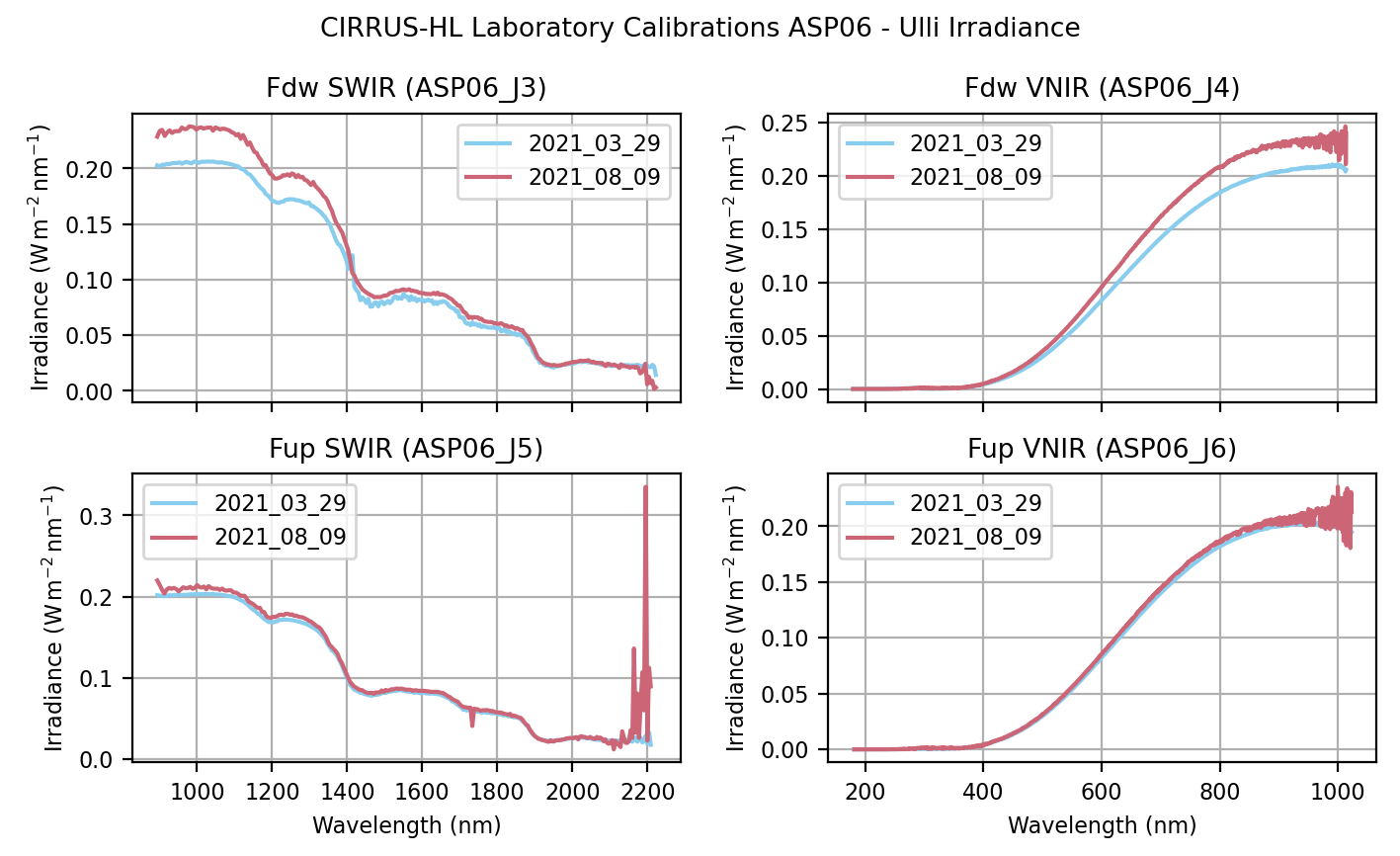
Fig. 48 Calculated irradiance of the Ulli transfer sphere from ASP06.

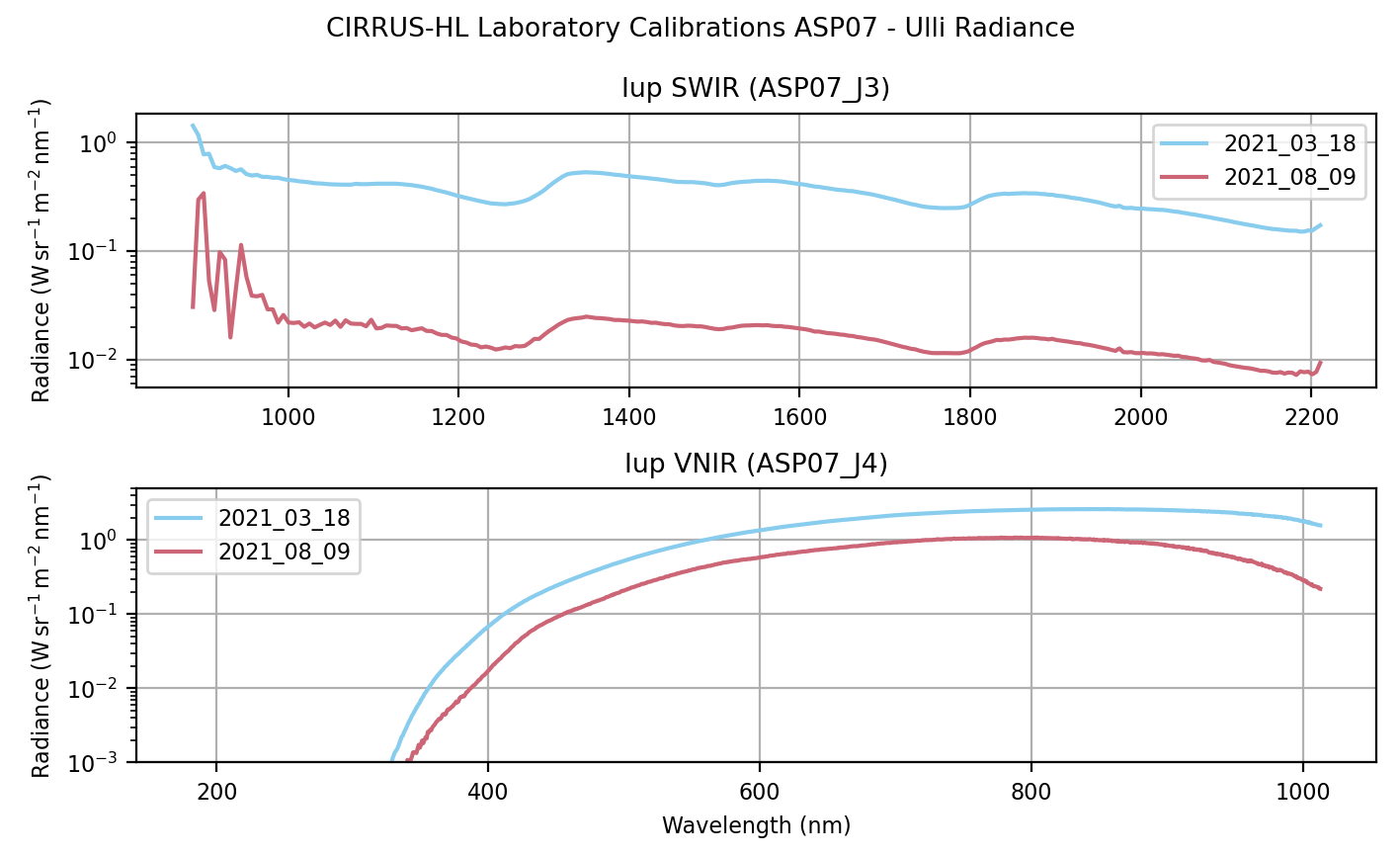
Fig. 49 Calculated radiance of the Ulli transfer sphere from ASP07.

Plotting the actual difference between the two shows a more detailed picture.

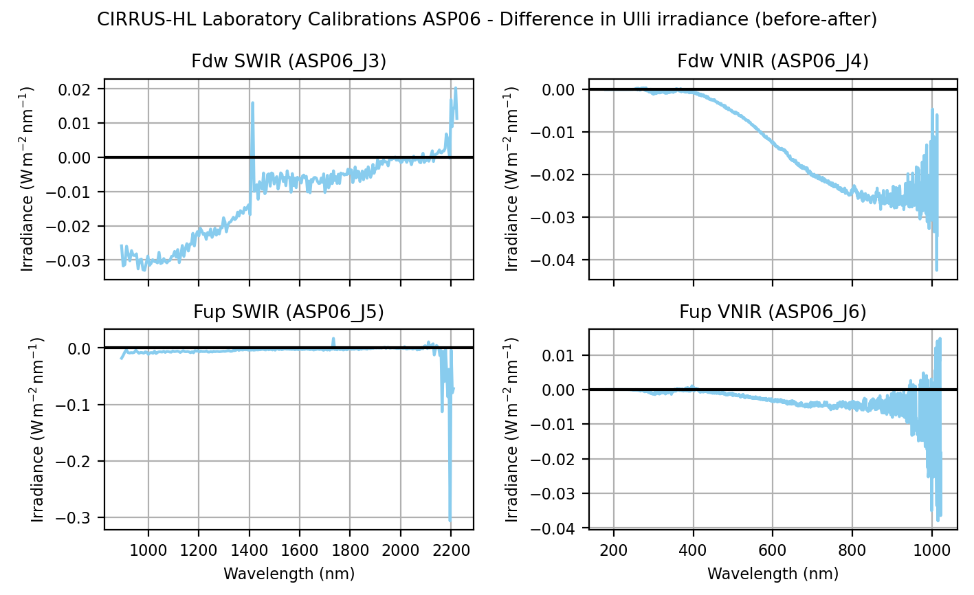
Fig. 50 Difference between measured irradiances from Ulli sphere (before - after).

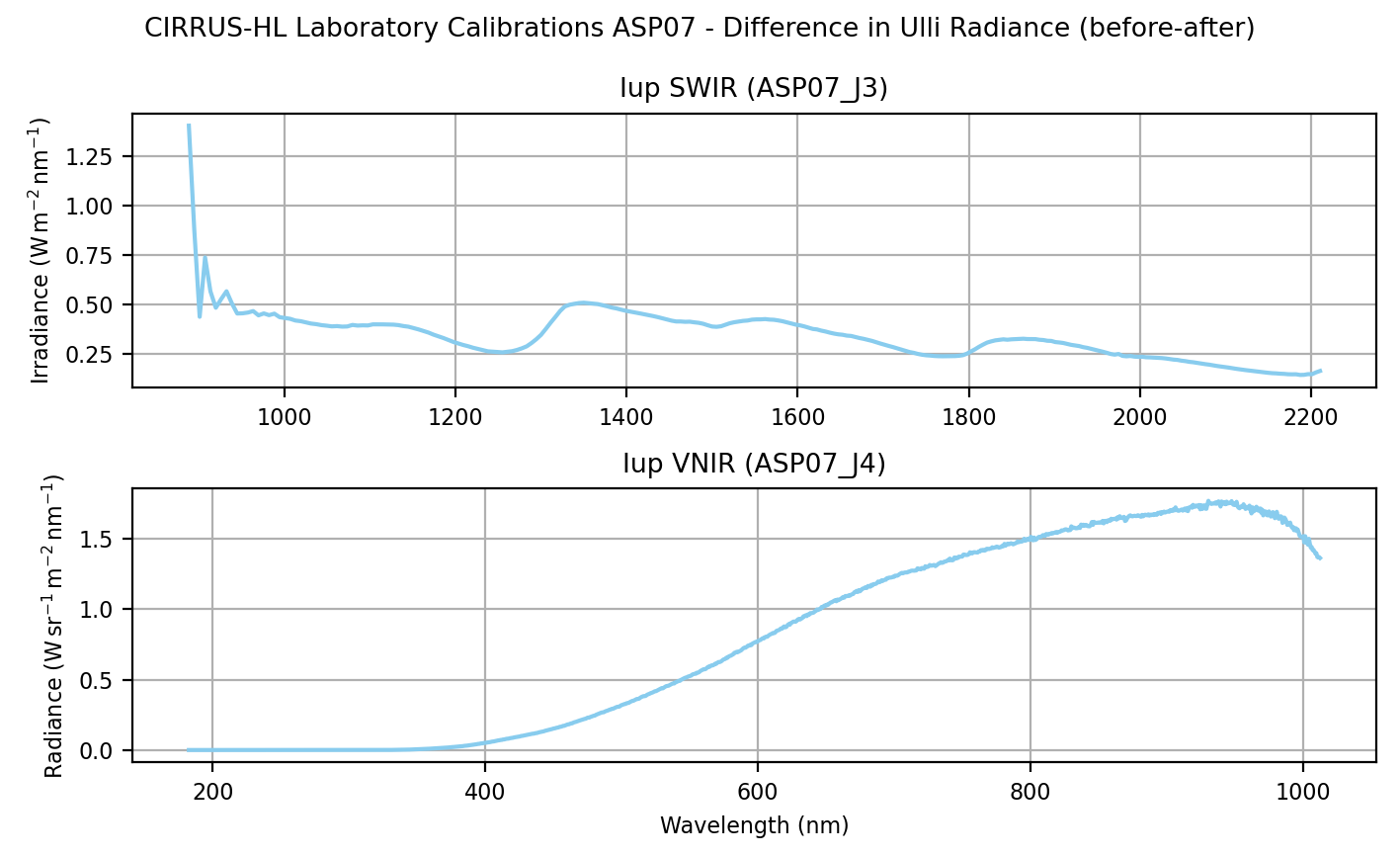
Fig. 51 Difference between measured radiances from Ulli sphere (before - after).

author: Johannes Röttenbacher

cirrus_hl_campaign_analysis.py

Analysis script for statistics about the whole campaign

author: Johannes Röttenbacher

cirrus_hl_case_study_20210625a.py

Case study for Cirrus-HL * 25.06.2021: Radiation Square for BACARDI author: Johannes Röttenbacher

cirrus_hl_case_study_20210629a.py

Case study for Cirrus-HL - 29. June 2021

Cirrus over Atlantic west and north of Iceland

-> Poster HALO Status Colloquium 2021 -> Presentation for CIRRUS-HL workshop 2. - 3.12.2021 -> 1. PhD Talk -> Presentation for CIRRUS-HL workshop 30. - 31.05.2022

author: Johannes Röttenbacher

cirrus_hl_case_study_20210712a.py

Case study for Cirrus-HL * 12.07.2021: First day with SMART fixed author: Johannes Röttenbacher

cirrus_hl_case_study_20210715a.py

Case study for CIRRUS-HL Flight_20210715a

• 15.07.2021 SMART fixed - contrail outbreak over Spain - Radiation Square

See CIRRUS-HL_radiation_square_SMART.pptx in campaigns/CIRRUS-HL/case_studies/Flight_20210715a for results.

author: Johannes Röttenbacher

cirrus_hl_overview.py

Prepare overview plots for each flight author: Johannes Röttenbacher

HALO-(AC)³

HALO-(AC)³ Laboratory Calibration comparison

Script: halo_ac3_smart_compare_lab_calibs.py

HALO-(AC)³: Compare laboratory calibrations of SMART

For HALO-(AC)³ two laboratory calibrations were done. Here the two calibrations are compared to each other.

Important: It was decided to use the other spectrometer pair (J5, J6) because the dark current looks better and does not have as many high offsets on some pixels. Also see the note on the effective receiving area! Due to technical difficulties the spectrometer pair J3, J4 was used during HALO-AC3. This calibration was therefore used for the transfer calibration. However, a different inlet was used (VN05). The first calib was done with inlet VN11.

Note on effective receiving area: Effective receiving area is in front of inlet not inside it, but was interpreted otherwise. Thus, the distance between the effective receiving area and the lamp is off by 44mm!

Timeline

• 15.11.2021: First lab calibration before → Used wrong inlet VN11, channels J3 and J4, assumed wrong effective receiving area

• 23.11.2021: Second lab calibration before → Used wrong inlet VN11, channels J5 and J6

• 15.02.2022: First transfer calibration in Oberpfaffenhofen with Ulli2 (packed in container for Kiruna afterwards) and Ulli3 (stays in Oberpfaffenhofen) using VN05 and J5 and J6

• 21.02.2022: EMI test flight → J3, J4

• 22.02.2022: saved new offsets for SMART stabilization, transfer calibration with Ulli2 and multiple integration times → J5, J6

• 25.02.2022: Scientific test flight → J5, J6

• 11.03.2022: Transfer flight to Kiruna → J3, J4

• 13.03.2022: First transfer calibration in Kiruna → J3, J4

• 11.04.2022: Final transfer calibration in Kiruna

• 02.05.2022: Transfer calibration in lab in Leipzig (optical fibers were detached from Spectrometers in between)

• 02.05.2022: Laboratory calibration after campaign → VN05, channels J3 and J4

• 06.05.2022: Wavelength calibration

The second lab calibration after the campaign was done with the correct inlet and the correct channels: VN05 and J3, J4

Each lab calibration is processed with smart_process_lab_calib_halo_ac3.py to correct the files for the dark current. After that the calibration factors are calculated with analysis.smart_calib_lab_ASP06_halo_ac3.py for ASP06.

• compare calibration factors

• compare Ulli measurements

Results HALO-(AC)³

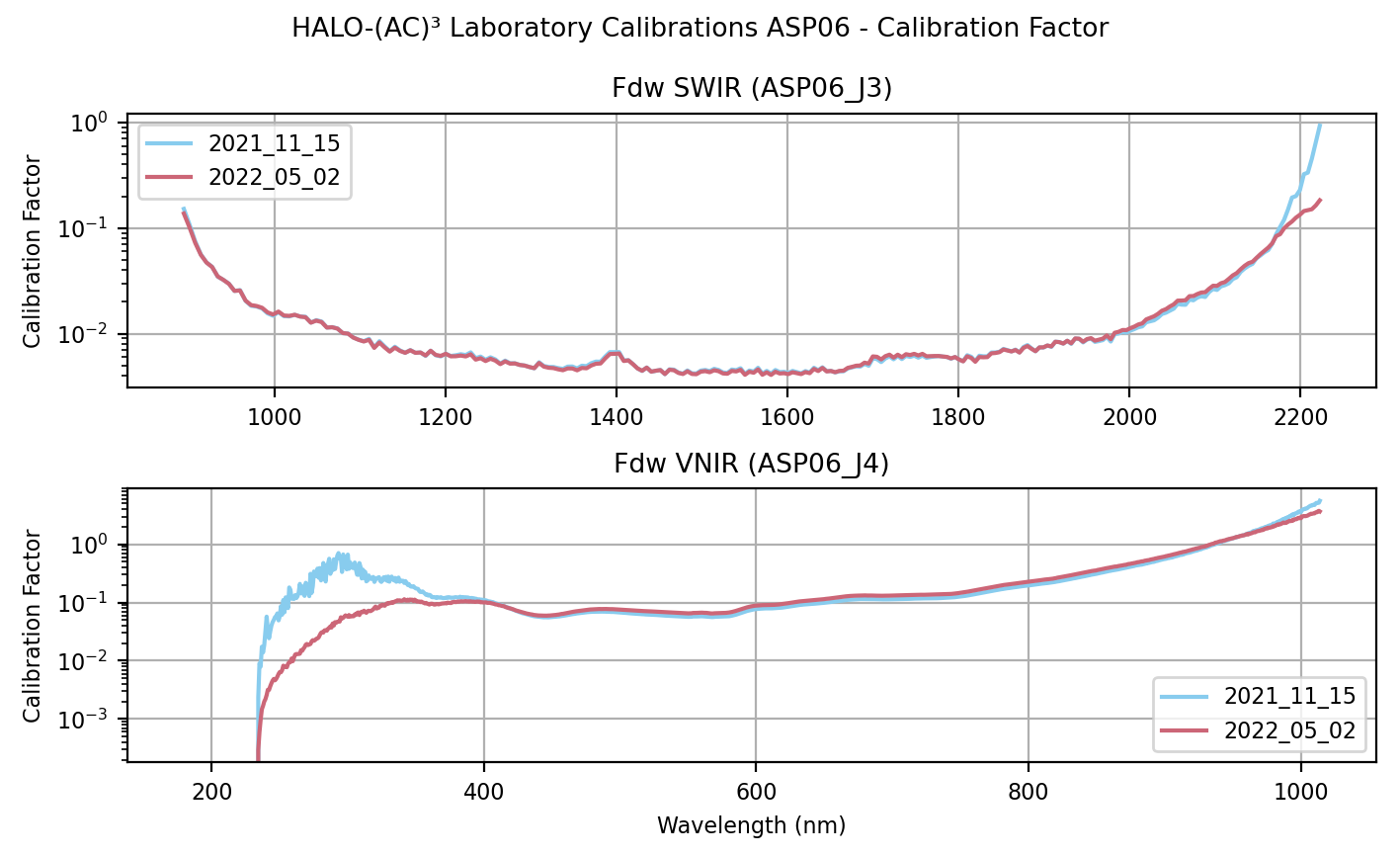
Fig. 52 Comparison of the lab calibration factors before and after HALO-(AC)³ for the two channels on ASP06.

Comparing the calibration factors of ASP06 between the before and after calibration shows that the after calibration (red) has a lower magnitude in the wavelength range from 250 to 350 nm for the VNIR channel. This means less signal in the before calibration for those pixels.

Ulli measurements

Taking a look at ASP06’s measurements of the Ulbricht sphere (Ulli2) shows only a minor difference in magnitude between the calibrations when comparing the dark current corrected and normalized counts. Especially in the VNIR part between 180 and 350nm a lot of noise can be seen, which might already explain the difference in calibration factors for those wavelengths.

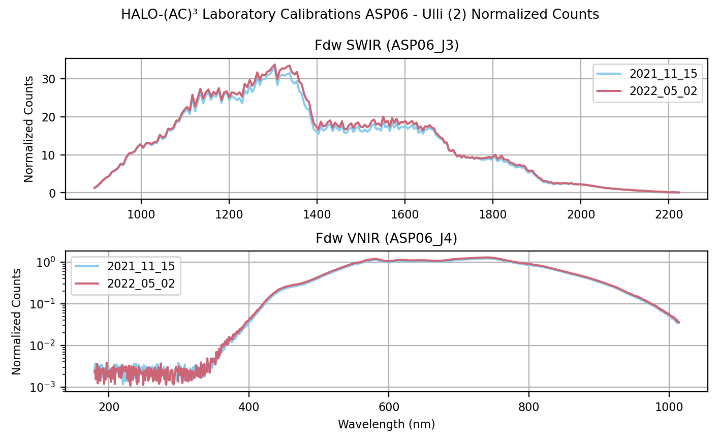
Fig. 53 Dark current corrected, normalized count measurements of the Ulli transfer sphere (Ulli2) from ASP06.

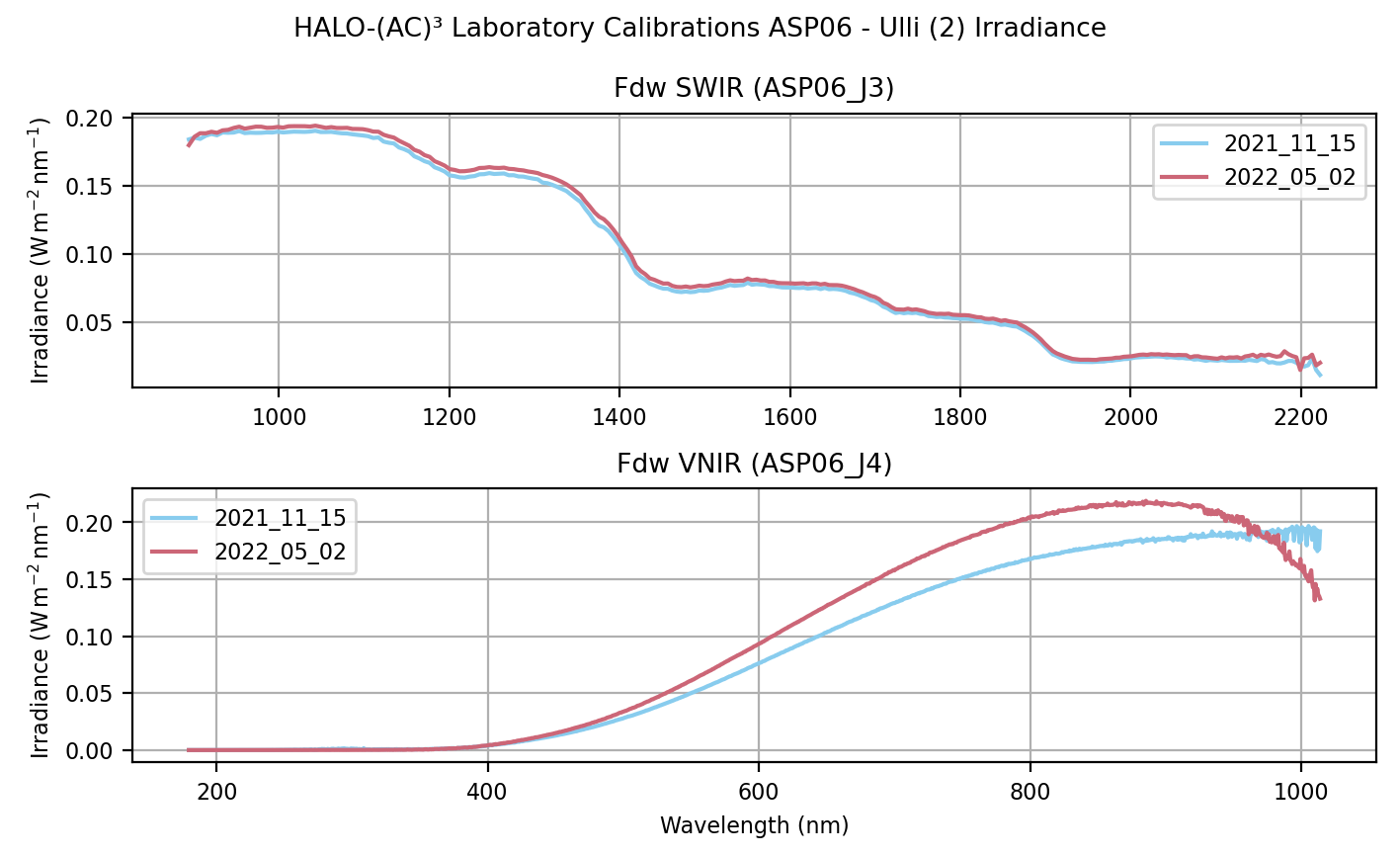
Fig. 54 Calculated irradiance of the Ulli transfer sphere (Ulli2) from ASP06 measurements.

Plotting the actual difference between the two shows a more detailed picture.

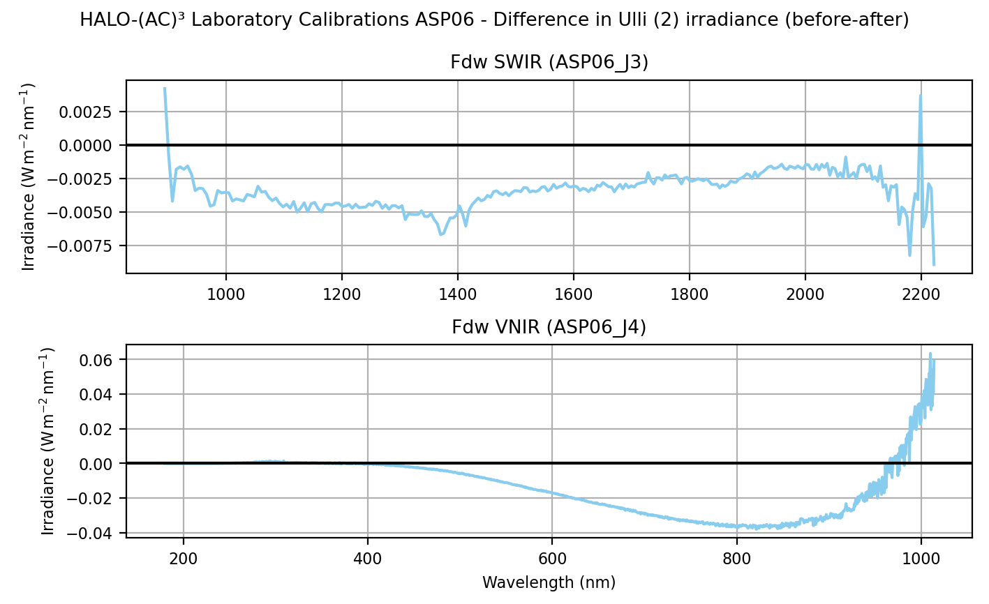
Fig. 55 Difference between measured irradiances from Ulli sphere (Ulli2) (before - after).

The after campaign calibration shows a higher irradiance with increasing wavelength in the VNIR channel (J4).

There were several problems with the before calibration on 15. November 2021:

• wrong inlet used (VN11 instead of VN05)

• the effective receiving area was wrongly interpreted leading to an offset of 44mm in the distance between the calibration lamp and the inlet (should be 50cm)

• the power supply for Ulli3 had a voltage limit in place instead of a current limit → only relevant for the transfer calibration at Oberpfaffenhofen before the campaign

Thus, it is decided to use the after campaign calibration for all transfer calibrations.

author: Johannes Röttenbacher

HALO-(AC)³ Transfer Calibrations

Script: halo_ac3_smart_check_transfer_calibrations.py

Go through all transfer calibrations and check the quality of the calibration

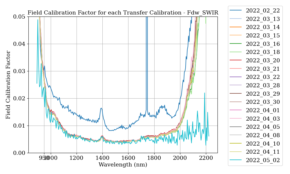
Fig. 56 Field calibration factors for all transfer calibrations using the after campaign lab calibration.

It can be seen that the first and last transfer calibration result in quite different calibration factors. However, the first transfer calibration was done with different spectrometers and the last transfer calibration happened after the optical fibers were detached and reattached to the spectrometers. The difference is thus not surprising. The performance of the spectrometers throughout the campaign was stable. Judging from the steep increase in the field calibration factor at the borders of the spectrometers 950 nm seems to be a reasonable wavelength to switch from VNIR to SWIR for the combined output data.

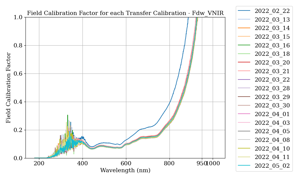
Fig. 57 Field calibration factors for all transfer calibrations using the after campaign lab calibration.

author: Johannes Röttenbacher

HALO-(AC)³ SWIR Offset Investigation

Script: halo_ac3_smart_SWIR_offset_investigation.py

Investigate offset of SWIR spectrometer during HALO-(AC)³

After the first final calibration for HALO-(AC)³ (September 2022) it was discovered that the SWIR spectrometer data consistently shows too low values compared to the VNIR spectrometer. The VNIR spectrometer is closer to the libRadtran clearsky simulation and can thus be considered to be “true”. To investigate this offset RF14 is used as it was a flight with a lot of long straight legs. One of which was heading far north and thus experiencing high solar zenith angles.

Steps:

• Checked all SWIR dark current → no change over flight (see .../quicklooks/SMART_SWIR_dark_current)

• VNIR dark current comes from transfer calibration → looks good (see Fig. 58)

• Plot minutely averaged spectra → offset between spectrometers gets smaller with higher wavelengths (see .../case_studies/...RF14/spectra)

• Check mean difference between VNIR and SWIR for different wavelengths (see Table 2)

• Look at other flights and plot the spectra of those (RF17)

• look at difference between VNIR and SWIR for 985nm for all flights (see Fig. 61)

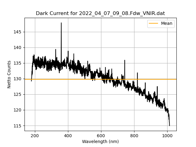
Fig. 58 Dark current used for correction of VNIR measurements during RF14.

Dark current correction works as expected. The dark current is also correctly written into the calibrated netCDF files. The field calibration factor looks stable between 950 and 2100 nm for the SWIR spectrometer. The VNIR field calibration factor shows a strong increase towards higher wavelengths.

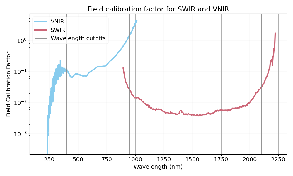
Fig. 59 Field calibration factor for the VNIR and the SWIR spectrometer for RF14. Wavelength cutoffs at 400, 950 and 2100 nm.

Looking at minutely averaged spectra from both spectrometers shows that the offset between the two is less for higher wavelengths. Thus, 975nm is tried as a cutoff between the two. The difference between the two 975nm measurements is shown below. It can be seen that the VNIR spectrometer is usually between 0.02 and 0.05 \(W\,m^{-2}\,nm^{-1}\) higher than the SWIR spectrometer.

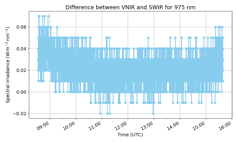
Fig. 60 Difference between VNIR and SWIR spectrometer for 975nm during RF14. Exact wavelengths differ slightly, 974.8nm and 972.8nm (VNIR, SWIR).

Looking at different wavelengths and calculating the mean difference yields the following results fro RF14.

Table 2 Mean difference between selected wavelengths measured with the VNIR and the SWIR spectrometer at the closest corresponding wavelength fro RF14.

Wavelength	VNIR wavelength	SWIR wavelength	Mean difference
950	949.72	946.88	0.029
955	954.80	953.39	0.026
960	959.85	959.88	0.028
965	964.85	966.36	0.020
970	969.82	972.81	0.016
975	974.75	972.81	0.021
980	980.34	979.25	0.012
985	985.18	985.68	0.008
990	989.98	992.09	0.013
995	994.73	992.09	0.010
990	989.98	992.09	0.013
995	994.73	992.09	0.010

The mean difference between 985nm is lowest. At this wavelength also the VNIR and SWIR wavelengths are close to each other, only 0.5nm difference. However, at 960nm the difference is only 0.08nm but the difference in measurement is 0.028 \(W\,m^{-2}\,nm^{-1}\).

The analysis is repeated for each flight and the difference between the 985nm pixel from the two spectrometers is shown in Fig. 61. The single txt files for all wavelengths for one flight can be found in the respective case study folders. One csv file with all flights has been saved in the case_studies folder (mean_diff_VNIR-SWIR.csv).

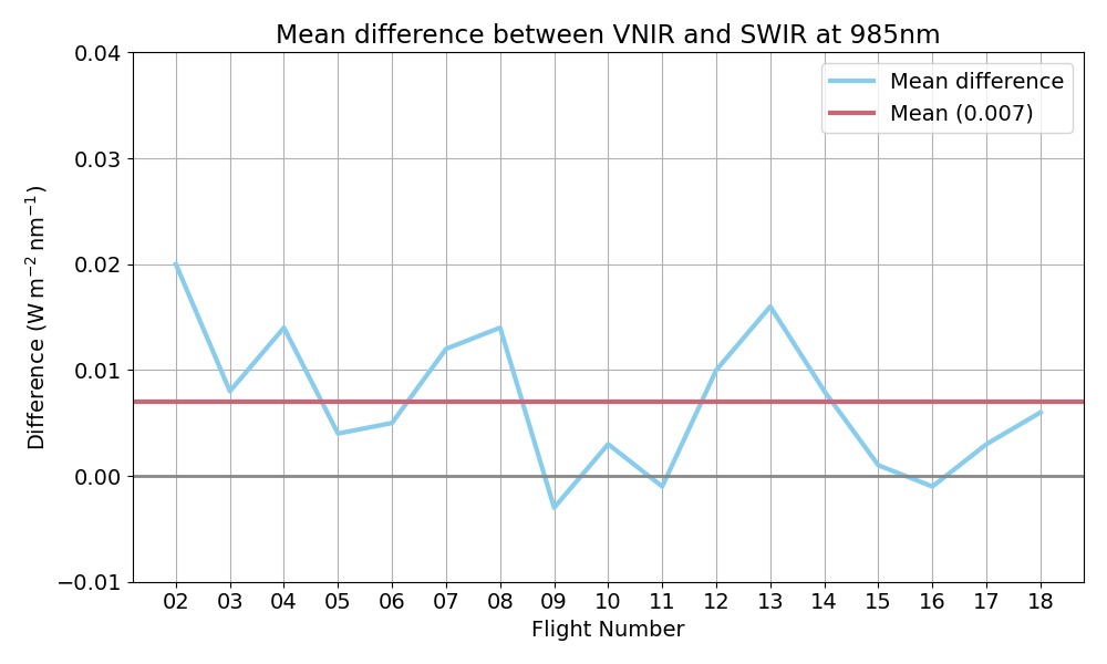
Fig. 61 Mean difference between the 985nm measurement from the VNIR (985.18nm) and the SWIR (985.68nm) spectrometer for each research flight.

This plot is produced for each wavelength between 950 and 995nm. They can be found in .../case_studies/spectrometer_overlap. Looking through those plots it becomes apparent that the 990nm wavelength shows the lowest difference between the two spectrometers on average.

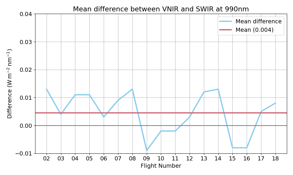
Fig. 62 Mean difference between the 990nm measurement from the VNIR (989.98nm) and the SWIR (992.09nm) spectrometer for each research flight.

Due to this result the wavelength at which the two spectra are merged is set to 990 nm.

author: Johannes Röttenbacher

HALO-(AC)³ Radiation Square Investigation 2022-04-12

Script: halo_ac3_smart_case_study_20220412_radiation_square.py

Find correction offsets for SMART

During RF18 the SMART INS system had an error and the stabilization had to be fixed to keep on measuring. Looking at the stabilization table measurements one can see the values start to drift after the stabilization was turned on again after the radar calibration maneuvers.

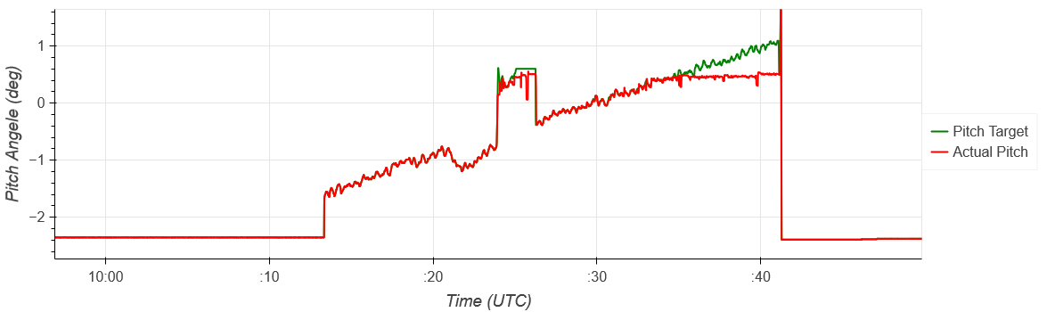
The stabbi was turned on again at 10:13:22. And shortly after (10:35 UTC) the stabilization table was fixed to the following position:

• Roll 0.07

• Pitch -2.38

This should account for the usual position of the aircraft in flight. (HALO’s nose is usually pointing a bit up during flight thus the table needs to counter this)

Looking at the BAHAMAS data filtered for roll angles greater 1 we can see that leg two in the polygon shows some high roll angles. Fig. 63 also shows that the heading did not stay constant during each leg.

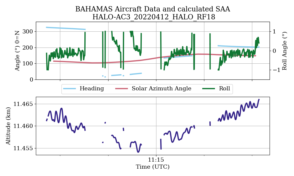
Fig. 63 BAHAMAS aircraft data filtered for roll angles greater 1 and the calculated solar azimuth angle (first row). BAHAMAS altitude (second row).

During the time when SMART was fixed in position the incoming direct solar irradiance can be corrected for the aircraft attitude. This correction can take an offset between the fixed position of SMART and the aircraft fuselage into account. To figure out this possible offset one can use a so-called radiation square where HALO flies into four different direction. Ideally HALO would fly once towards the direction of the sun and then do three 90 degree turns. From this pattern one can figure out the offset. However, here we only have a polygon pattern at hand with less than 90 degree turns and also did not fly directly into the direction of the sun (see Fig. 64).

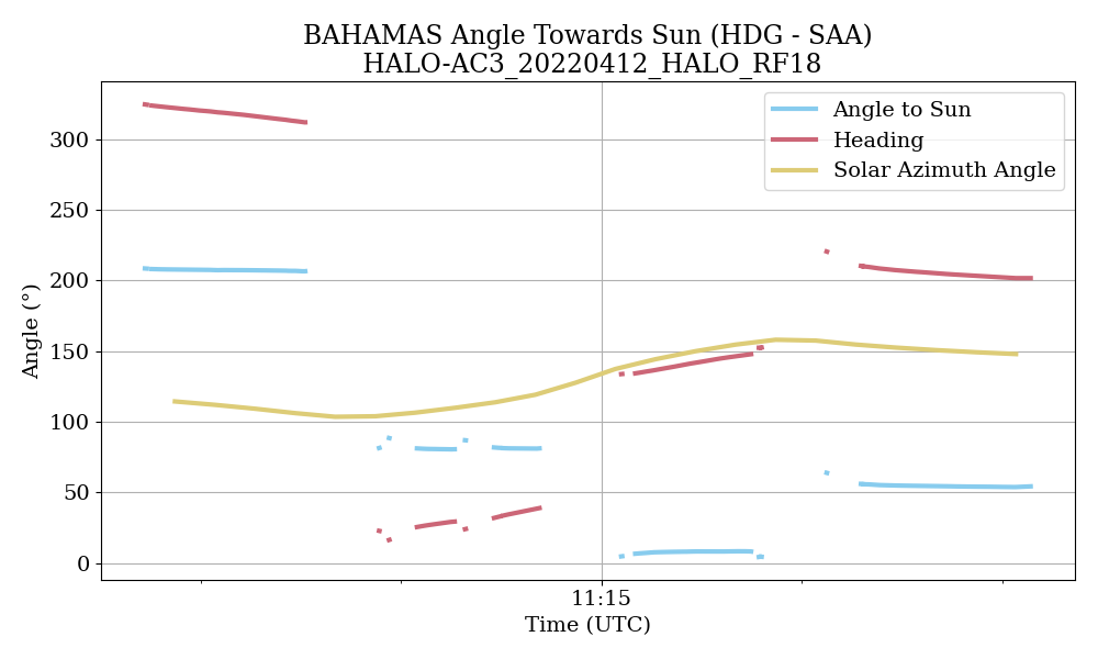
Fig. 64 Angle of HALO towards sun during the polygon pattern and BAHAMAS heading (HDG) and solar azimuth angle (SAA).

Using the Jupyter notebook halo_ac3_20220412_radiation_square_investiagtion.ipynb different offsets can be tried out using an interactive widget. Going through different offsets the fit to the simulation does not get better than using no offset. Thus, the inlet seems to be well aligned with the horizontal plane of the aircraft and no offset is applied to the attitude correction. Some plots can be found in .../case_studies/HALO-AC3_20220412_HALO_RF18/.

author: Johannes Röttenbacher

HALO-(AC)³ BACARDI Measurement Investigation

Script: halo_ac3_bacardi_measurement_investigation.py

BACARDI measurement investigation

Using RF17 the measurement performance of BACARDI is investigated. The data is filtered using motion angles measured by BAHAMAS. As the roll angle is centered around 0 (median for RF17: 0.0571659 deg) a simple roll threshold of 0.5 is used here and implemented by comparing the absolute roll angle with the threshold. The pitch angle of HALO, however, is centered on 2.28 (median for RF17: 2.28605413 deg) and thus the absolute value of the measurement minus the center is compared with the pitch threshold of 0.34. The pitch threshold is set by iterating the polar plot showing the relation between the BACARDI measured downward irradiance and the libRadtran clearsky simulation according to viewing angle of HALO (see Fig. 65). There is one point in the dataset which shows an abnormal low relation. This point is removed when the pitch threshold is set to 0.34. It can thus be said that the low relation value is caused by a pitch motion of HALO.

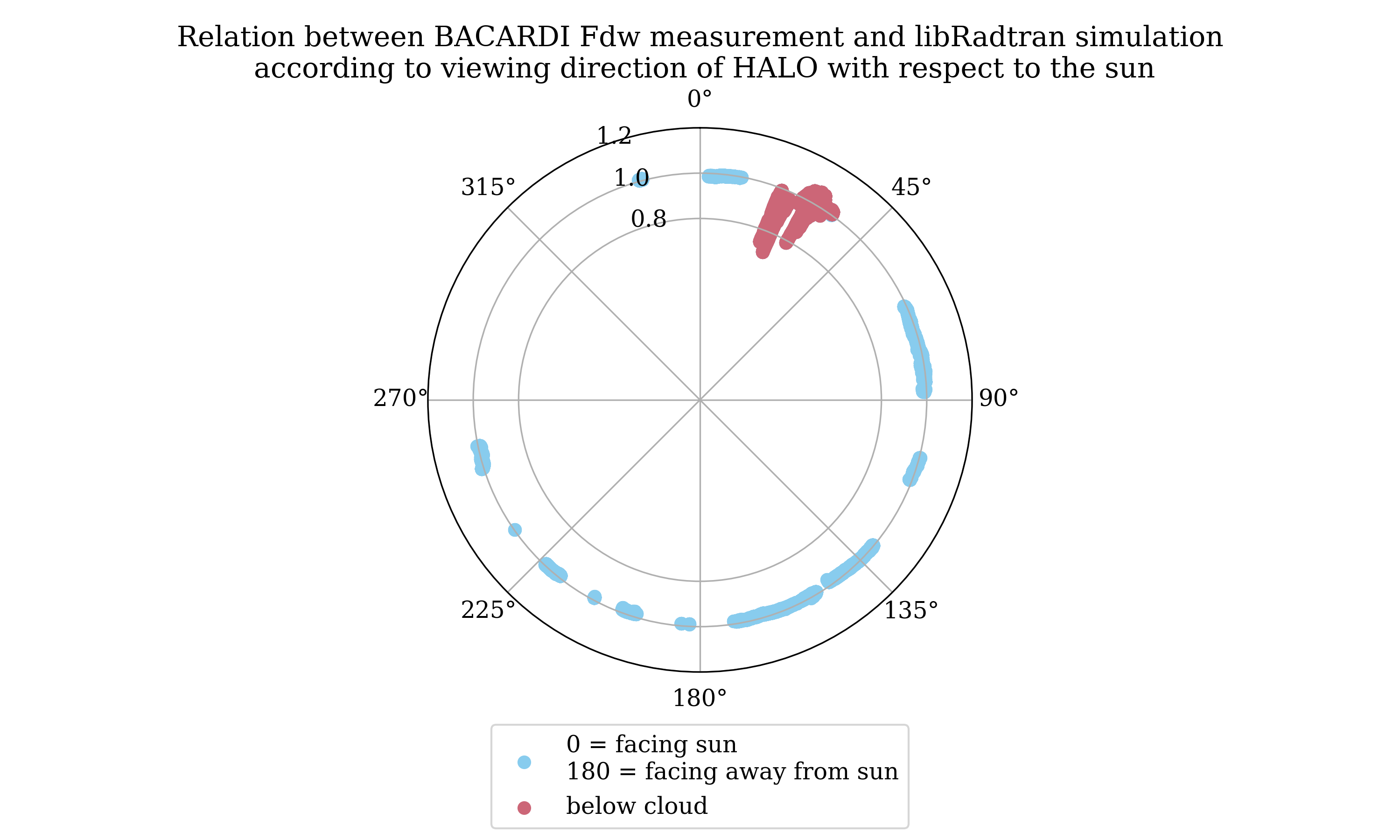
Fig. 65 Relation between BACARDI measurement and libRadtran clearsky simulation depending on viewing direction of HALO. BACARDI data is filtered for aircraft motion. Red dots denote the section when HALO was below a cirrus cloud.

Plotting the same relation against the solar zenith angle (Fig. 66) shows that there is some part of the flight when the relation exceeds 1 and HALO is above any cloud. However, due to the below cloud section not many details can be observed.

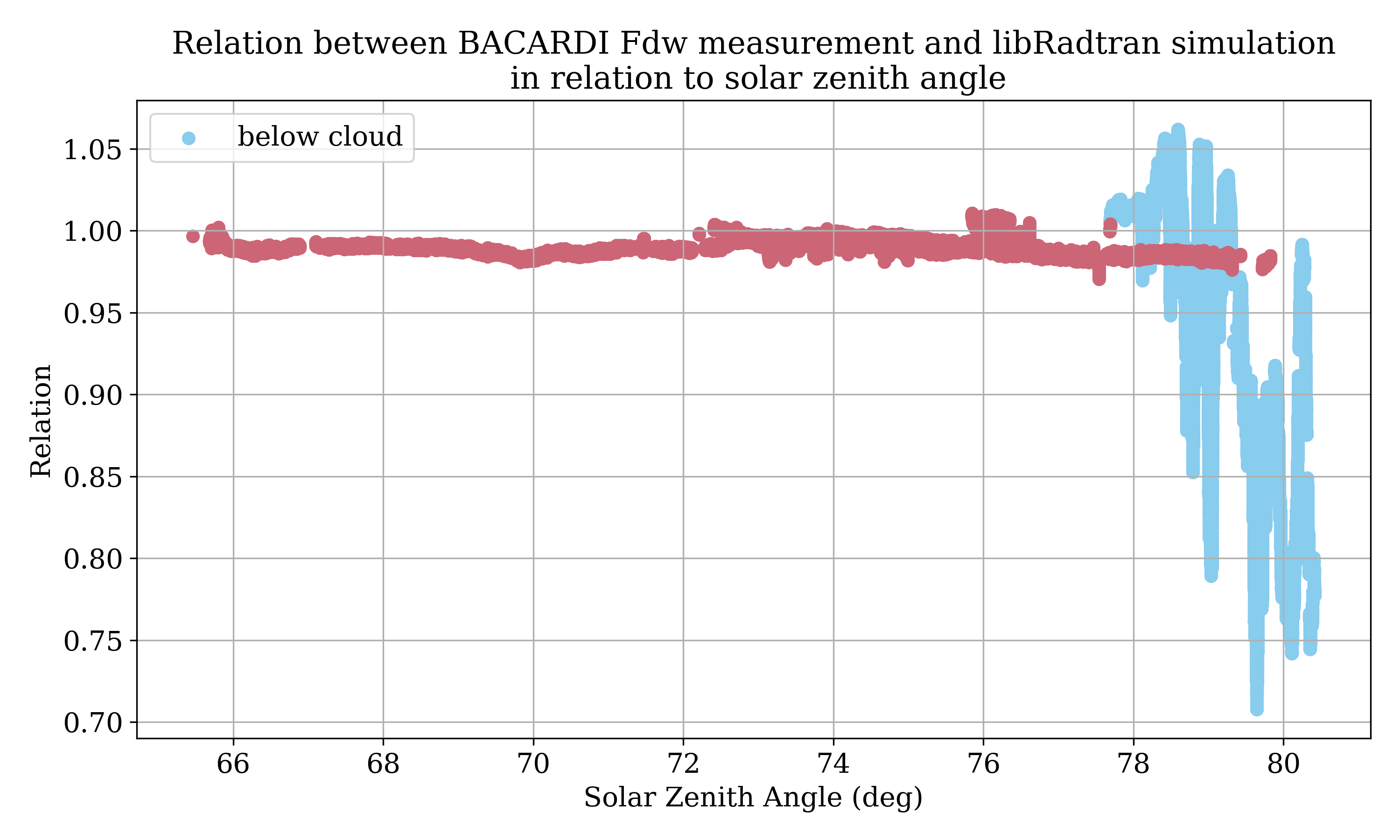
Fig. 66 Relation between BACARDI measurement and libRadtran clearsky simulation depending on solar zenith angle. BACARDI data is filtered for aircraft motion. Blue dots denote the section when HALO was below a cirrus cloud.

More details can be seen in Fig. 67. Here a maximum deviation of 3% can be observed, which is not much considering the motion thresholds.

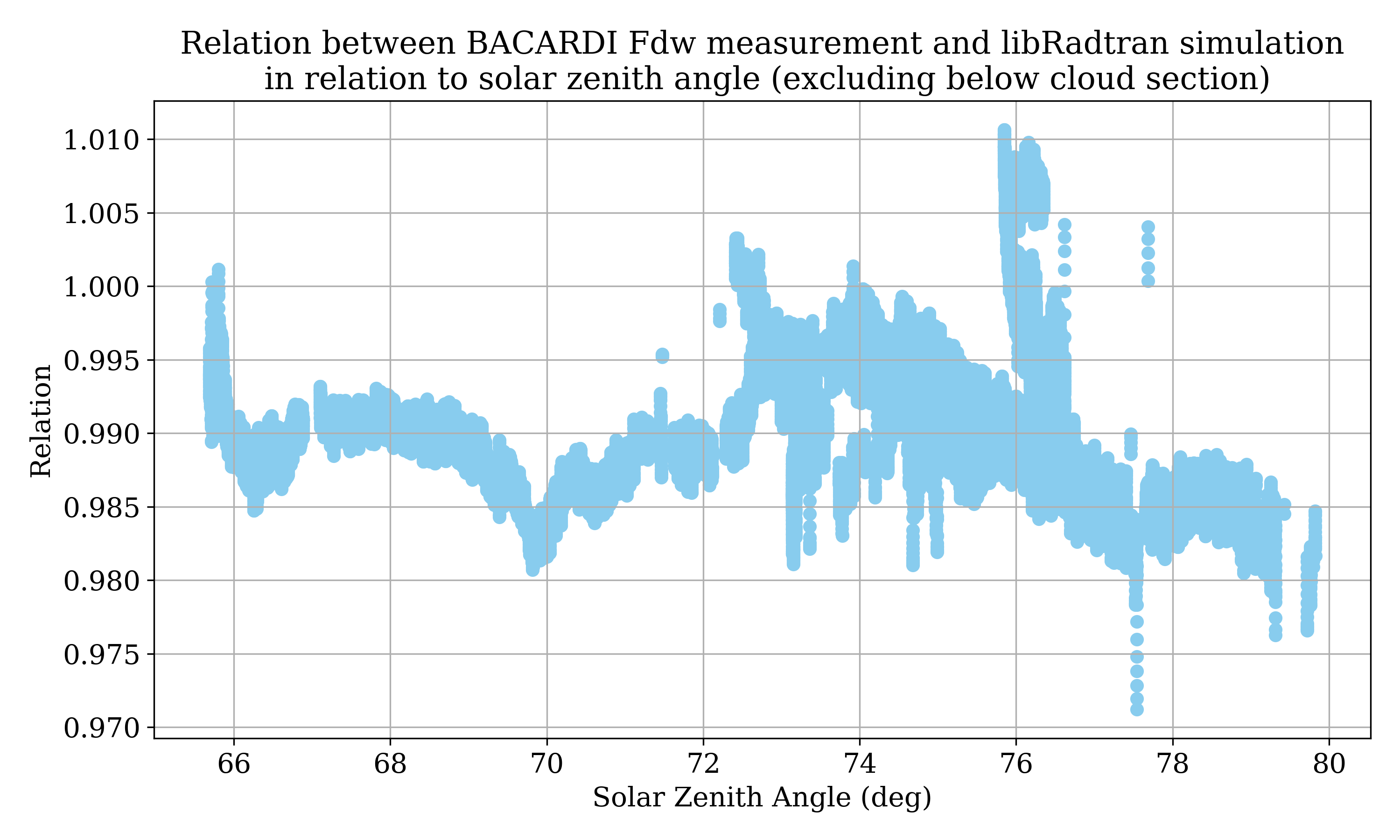
Fig. 67 Relation between BACARDI measurement and libRadtran clearsky simulation depending on solar zenith angle. BACARDI data is filtered for aircraft motion and the below cloud section.

Looking at the time evolution of the relation (Fig. 68) we can see that the high deviations happen close to times when the data is filtered due to high motion angles and just before the start of the below cloud section.

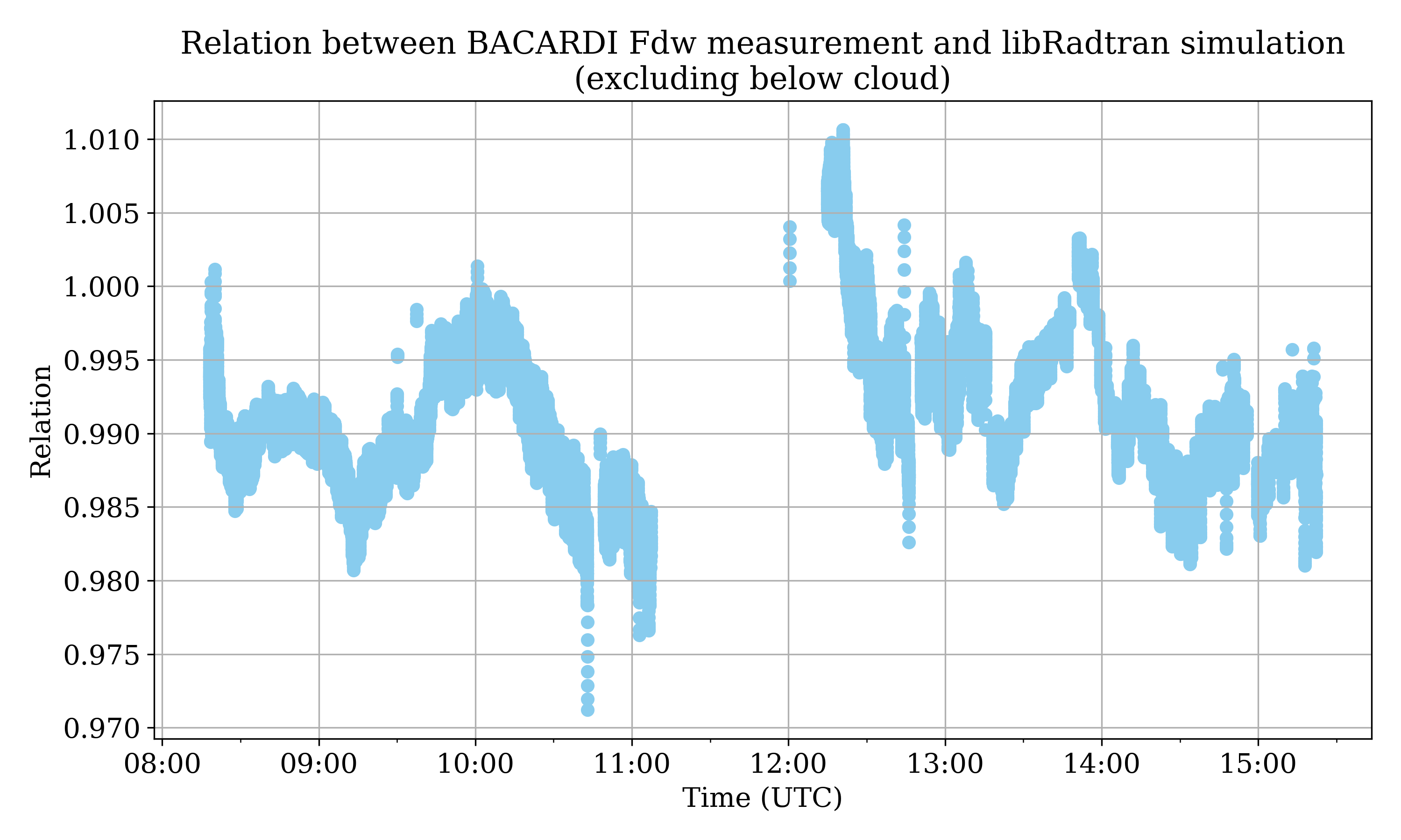
Fig. 68 Relation between BACARDI measurement and libRadtran clearsky simulation depending on time. BACARDI data is filtered for aircraft motion and the below cloud section.

author: Johannes Röttenbacher

HALO-(AC)³ BAHAMAS Pitch Filter Assessment

Script: halo_ac3_bahamas_pitch_filter.py

author: Johannes Röttenbacher

created: 20-02-2023

Investigate pitch angle of HALO measured by BAHAMAS during HALO-(AC)³

HALO’s pitch angle changes during the flight as it loses weight by burning fuel or when it changes altitude and speed. Using a static median pitch value to calculate a pitch threshold for motion filtering measurements is thus not sufficient. This can be seen in Fig. 69, where the ten-minute median pitch angle decreases from 2.8° to 1.8° during RF18. Using the static pitch thresholds would thus filter the wrong values. Especially, the above cloud section during the pentagram pattern in the far north, denoted as case study, suffers from this static threshold. However, Fig. 69 already shows a problem with a rolling median: During large ascents and descents the median follows the extreme values. One could either use an absolute threshold for such extreme values or look at the change of pitch over time to filter such events. The flight segmentation could also help to remove these events. Using a longer time window also shows good results.

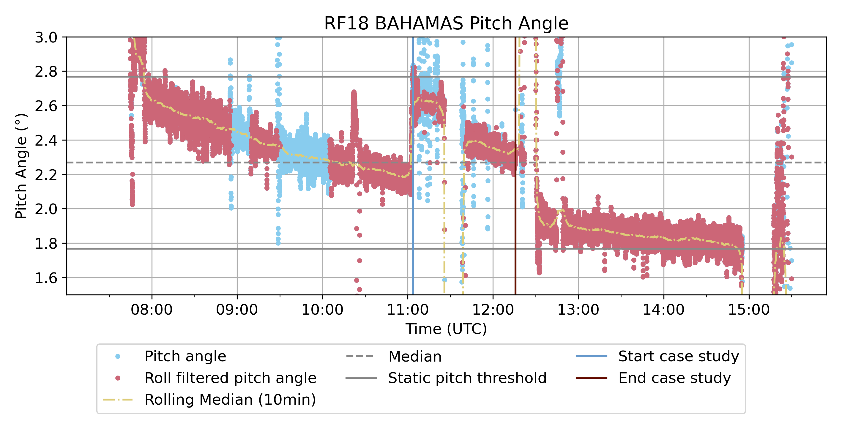
Fig. 69 BAHAMAS pitch angle during RF18 with whole flight median and 10 minute rolling median. Red dots show the roll filtered values.

Which time range is best for the median?

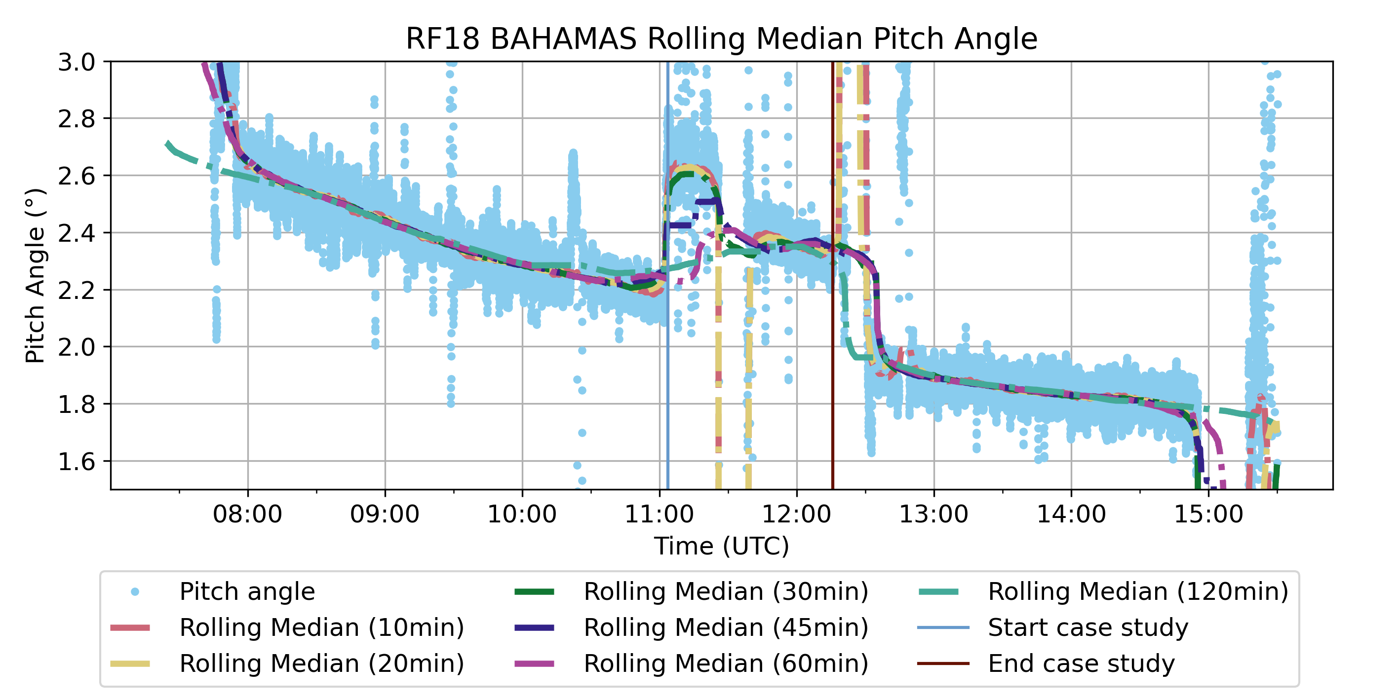
Fig. 70 Rolling median of pitch using different time windows.

Judging from RF18 30 minutes seem to be a good time window for the rolling median. Since it is mostly longer than large ascents and descents they are still averaged over. For case study like periods, however, it still follows the general trend of the data.

What threshold is best for the pitch?

To answer this we can have a look at the rolling standard deviation of the pitch in Fig. 71.

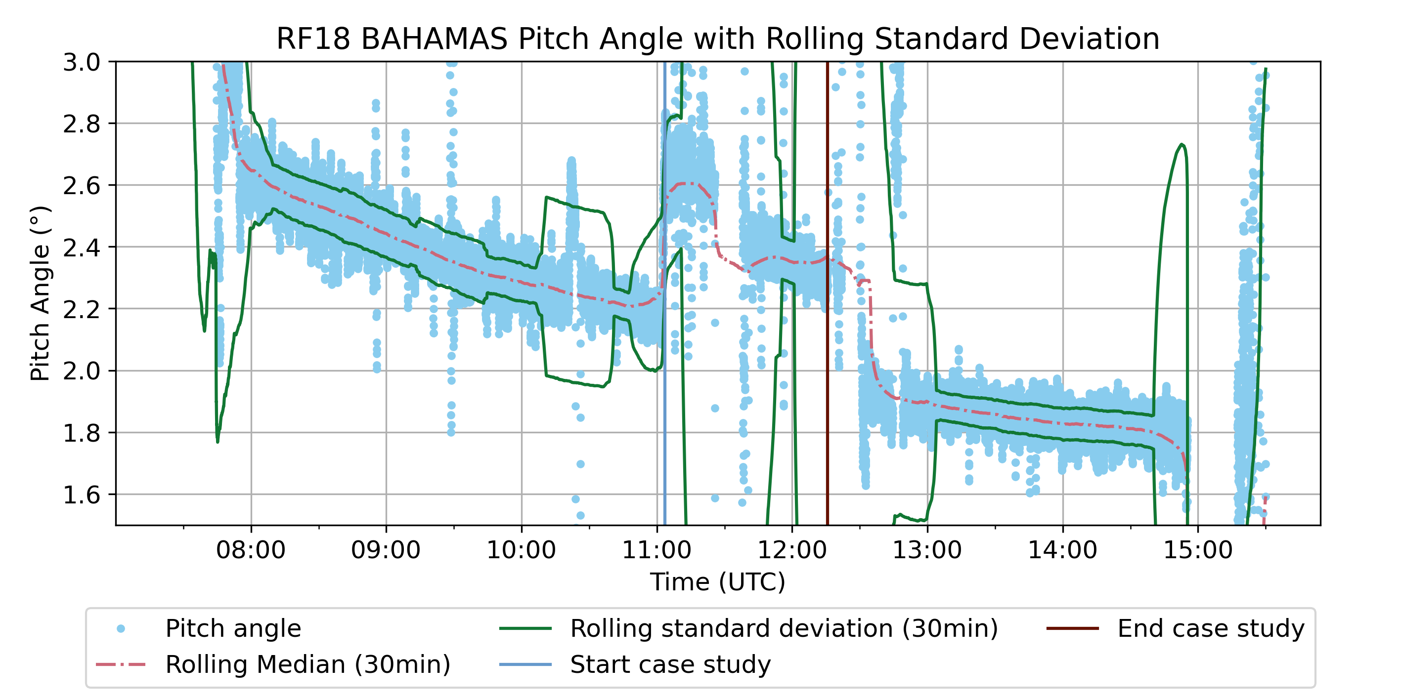
Fig. 71 Pitch and 30-minute rolling median pitch with standard deviation.

We see that the rolling standard deviation is actually quite small during time when HALO is flying steady. The median value of the 30-minute standard deviation is \(0.173^{\circ}\). Thus, \(0.17^{\circ}\) looks like a good threshold then. First result of calculating a dynamic pitch threshold can be seen in Fig. 72.

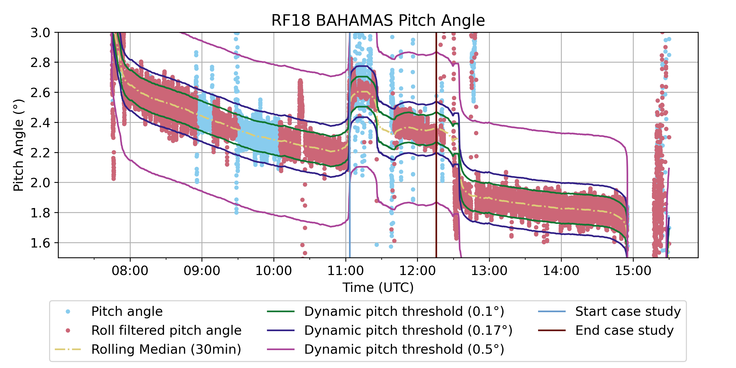
Fig. 72 Different dynamic pitch thresholds for a 30-minute rolling median.

From this we can see that the \(0.5^{\circ}\) threshold from the roll angle is too high for the pitch angle. The \(0.1^{\circ}\) threshold would cut off to many values during the steady flight sections.

Evaluation using BACARDI broadband measurements

BACARDI data is already filtered during the attitude correction. However, some errors remain as can be seen in Fig. 73.

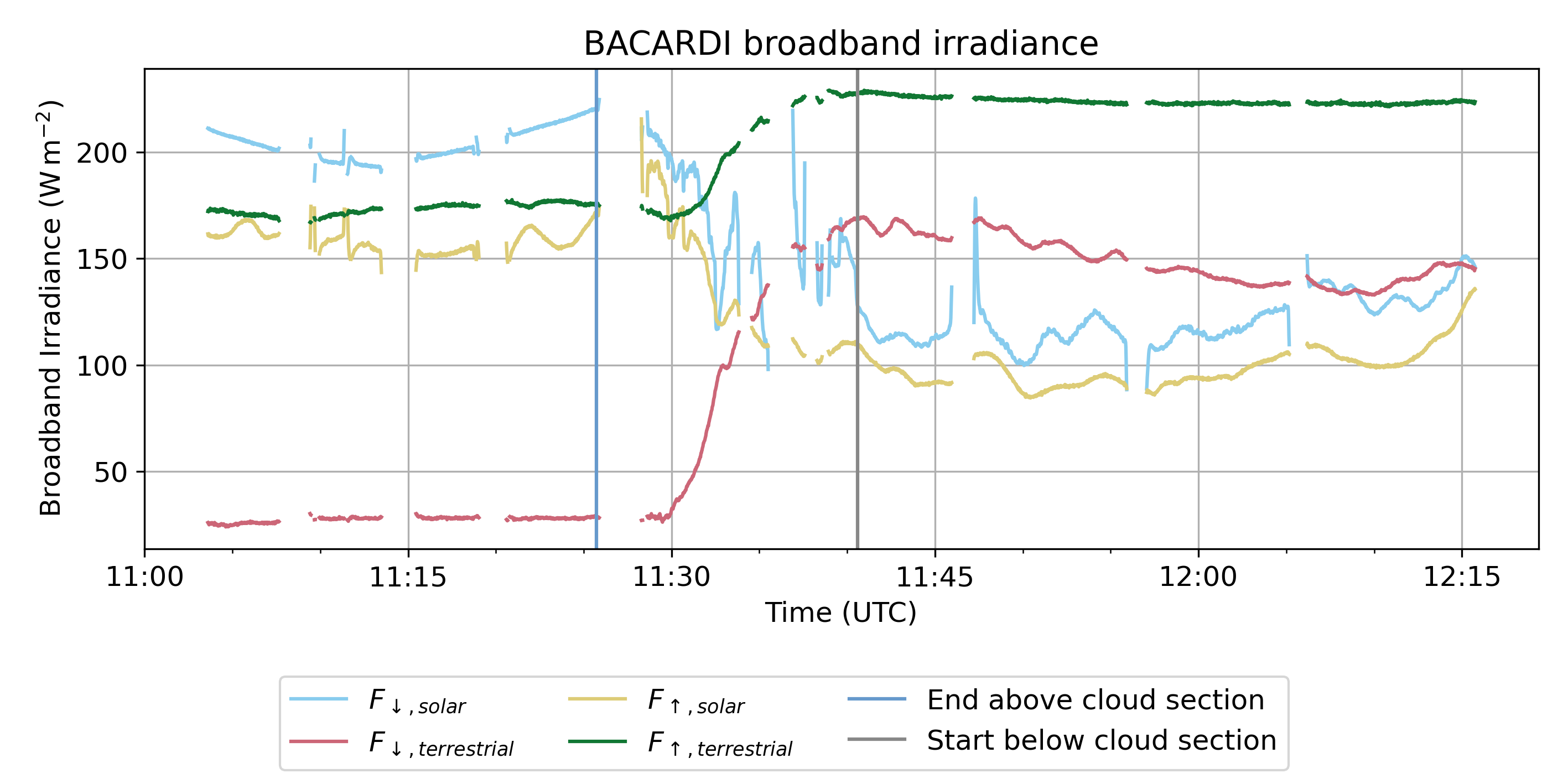
Fig. 73 Original filtered BACARDI values as returned from the calibration processing for the case study period. Note the peaks just before filters are applied.

HALO-(AC)³ ecRad VarCloud retrieval

Script: analysis.halo_ac3_case_study_ecrad_varcloud_v2.py

author: Johannes Röttenbacher

created: 12-07-2023

Comparison between using the VarCloud retrieval for IWC and \(r_{eff, ice}\) or the forecasted values from the IFS as input for an ecRad simulation using the Fu-IFS ice optic parameterization. In addition, an experiment is run where the above cloud retrieved IWC and \(r_{eff, ice}\) is used as input for the below cloud section. This allows for a comparison between measurements and simulations. The assumption is that the cloud does not change in the 30 minutes it takes to reach the below cloud section.

• IFS_namelist_jr_20220411_v15.nam: for flight RF17 with Fu-IFS ice model using IFS data from its original O1280 grid (input version v6)

• IFS_namelist_jr_20220411_v16.nam: for flight RF17 with Fu-IFS ice model using O1280 IFS data and varcloud retrieval for ciwc and re_ice input for the below cloud section (input version v7)

• IFS_namelist_jr_20220411_v17.nam: for flight RF17 with Fu-IFS ice model using O1280 IFS data and varcloud retrieval for ciwc and re_ice input (input version v8)

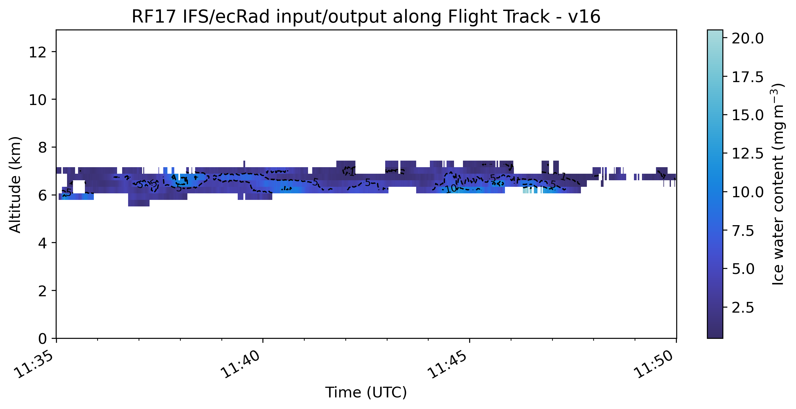
Fig. 74 Retrieved ice water content from VarCloud retrieval interpolated to IFS full level pressure altitudes.

Results

SMART

smart_cosine_calibration.py

Cosine Response Calibration of irradiance inlets of SMART for CIRRUS-HL and HALO-(AC)3

Deprecated since version 16.11.2021: The measurements were done with the inlets switched and not all measurements were performed so it was decided to repeat the whole calibration (see smart_cosine_calibration_v2.py). This script is kept for archiving only.

• ASP06 J3, J4 (Fdw) with inlet ASP02 done on 5th November 2021 by Anna Luebke and Johannes Röttenbacher

• ASP06 J6, J6 (Fup) with inlet ASP01 done on 8th November 2021 by Anna Luebke and Johannes Röttenbacher

Lamp used: FEL-1587

The inlet was rotated at 5° increments in both directions away from the lamp. Clockwise is positive. Each measurement lasted about 30 seconds with 1000 ms integration time. Data is stored in folders which denote the angle the inlet was turned to.

• angle_turned: The inlet was turned 90deg around the horizontal axis to evaluate all four azimuth directions

• angle_diffuse: A baffle was placed before the inlet to shade it (dark measurements)

author: Johannes Röttenbacher

smart_cosine_calibration_v2.py

Cosine Response Calibration of irradiance inlets of SMART for CIRRUS-HL and HALO-(AC)3 2nd try

• ASP06 J3, J4 (Fdw) with inlet VN05 (ASP_01) done on 16th November 2021 by Anna Luebke and Johannes Röttenbacher and finished on 22th November by Benjamin Kirbus and Johannes

• ASP06 J5, J6 (Fup) with inlet VN11 (ASP_02) done on 22th November 2021 by Benjamin Kirbus and Johannes Röttenbacher

Lamp used: cheap 1000W lamp optical fiber: 22b -> 21b has very little output from the SWIR fiber, thus the 22b fiber was chosen for both inlets as it is identical to 21b

The inlet was rotated at 5° increments in both directions away from the lamp. Clockwise is positive. Each measurement lasted about 42 seconds with 700 ms integration time for VN05 and about 48s with 800ms integration time for VN11. Data is stored in folders which denote the angle the inlet was turned to.

• angle_turned: The inlet was turned 90deg clockwise around the horizontal axis to evaluate all four azimuth directions

• angle_diffuse: A baffle was placed before the inlet to shade it (dark measurements)

Results Cosine Resopnse Calibration

See PowerPoint 20211122_SMART_cosine_calibration.pptx under instruments/SMART.

author: Johannes Röttenbacher

smart_effective_receiving_area.py

Calculate the effective receiving area of an irradiance inlet according to the R^2 law

author: Johannes Röttenbacher