Processing

With data processing one usually refers to the process of converting the raw measurement files as delivered by the instrument PC into error/bias corrected, calibrated and distributable/publishable files. For this work the netCDF standard is defined as the preferred output format.

Each instrument has different requirements before, after and during the campaign. In general these scripts are not meant for analysing the data to answer specific science questions or for producing quicklooks. This is handled by the scripts in the folders Analysis and Quicklooks.

SMART

SMART has to be calibrated in the lab and in the field so there are processing routines for both cases. Some scripts are designated for postprocessing specific campaign data as sometimes the normal processing does not cover all possible cases which occur during a campaign. In general scripts can be divided into Campaign Scripts and Postprocessing Scripts. The campaign scripts work under the assumption that everything worked as intended and are used in the field to quickly genrate calibrated data for quicklooks. The postprocessing scripts are campaign specific and try to correct for all eventualities and problems that occurred during the campaign.

Folder Structure

SMART data is organized by flight. Each flight folder has one SMART folder with the following subfolders:

• data_calibrated: dark current corrected and calibrated measurement files

• data_cor: dark current corrected measurement files

• raw: raw measurement files

Each campaign also has a calibration folder. In the calibration folder each calibration is saved in its own folder. Each calibration is used to generate one calibration file, which is corrected for dark current and saved in the top level calibration folder.

A few more folders needed are:

• raw_only: raw measurement files as written by ASP06/07, do not work on those files, but copy them into raw

• lamp_F1587: calibration lamp file

• panel_34816: reflectance panel file

• pixel_wl: pixel to wavelength files for each spectrometer

Workflow

There are two workflows:

1. Calibration files

2. Measurement files

Both workflows start with the correction of the dark current. After the raw files are copied from ASP06/07 into raw_only and raw the minutely files are corrected for the dark current and saved with the new ending *_cor.dat in data_cor. Then the minutely files are merged to one file per folder and channel.

Calibration files

Use smart_process_transfer_calib.py or smart_process_lab_calib_cirrus_hl.py to correct the calibration files for the dark current and merge the minutely files. Then run smart_calib_lab_ASP06.py or smart_calib_lab_ASP07.py for the lab calibrations or smart_calib_transfer.py for the transfer calibration. Each script returns a file in the calib folder with the calibration factors.

Measurement files

Use smart_write_dark_current_corrected_file.py to correct one flight for the dark current. Merge the resulting minutely files with smart_merge_minutely_files.py. Finally, calibrate the measurement with smart_calibrate_measurement.py. The resulting calibrated files are saved in the data_calibrated folder. As a final step the calibrated files can then be converted to netCDF with smart_write_ncfile.py.

Campaign Scripts

Measurement files

smart_write_dark_current_corrected_file.py

Script to correct all SMART measurements from one flight for the dark current and save them to new files

Set the input and output paths in config.toml.

Required User Input: campaign and flight(s)

Output: dark current corrected smart measurements

You can uncomment some lines to change the behavior of the script.

• run for all flights of a campaign

• run for one file

• correct a selection of files in a for loop and skip uncorrectable files

The default behavior is to run for one flight and execute everything in parallel. This is the campaign mode.

author: Johannes Roettenbacher

smart_merge_minutely_files.py

Script to merge minutely dark current corrected measurement files into one file per channel and folder.

Required User Input: campaign and flight

Output: one file with all dark current corrected measurements for one channel

ASP06 and ASP07 were configured to write minutely files. This script

• merges the minutely files into one file,

• deletes the minutely files,

• saves the merged files with the first found filename.

By uncommenting some lines you can switch between single flight (campaign mode) and multi flight mode.

author: Johannes Röttenbacher

smart_calibrate_measurement.py

Calibrate measurement files with the transfer calibration

Reads in dark current corrected measurement file and corresponding transfer calibration to calibrate measurement files.

Required User Input:

• campaign

• flight folder

• integration time of ASP06 and ASP07 measurements (check raw measurement files to get integration times)

• whether to normalize measurements or not (use normalized calibration factor, necessary if no calibration with the same integration time was made)

Output: Calibrated SMART measurement files in .dat format

author: Johannes Roettenbacher

smart_write_ncfile.py

Given a SMART input file write a well documented quicklook netCDF file.

Required User Input:

• campaign

• date

• flightkey

• property and channel (Fdw/Fup and SWIR/VNIR)

• uncomment import of metadata information depending on campaign

Output: Calibrated and documented netCDF file

Two options:

1. One spectrometer = one file

2. One flight = one file

Option 2 might result in a huge file but would be easier to distribute. With option 1 one could still merge all single files quite easily with xarray. Go with option 1 for now.

The netCDF file could be writen as a standard output from smart_calibrate_measurement.py or as a separate step in this script. Stick with this script for now.

author: Johannes Röttenbacher

Calibration files

smart_process_transfer_calib.py

Script to correct SMART transfer calibration measurement for dark current and save it to a new file and merge the minutely files

Required User Input: transfer calibration folder and campaign

Output: dark current corrected and merged smart measurements

author: Johannes Röttenbacher

smart_calib_transfer.py

Script to calculate field calibration factor and save a file for each PC and channel

Required User Input:

• campaign

• transfer calibration folder → should be found in calib folder

• laboratory calibration date to relate transfer calibration to

• integration time of transfer calibration (T_int) in ms

• whether to normalize the measurement by the integration time or not

Output: transfer calibration file with field calibration factor c_field (unit: \(W\,m^{-2}\, count^{-1}\))

Steps:

1. set user defined variables and list field calibration files and lab calibration files

2. for each field cali file:

   1. read field file and corresponding lab calibration file

   2. calculate field calibration factor and the relation between lab and field counts of the ulli sphere

   3. plot transfer calib measurements and save the plot

   4. save transfer calibration file in calib folder

author: Johannes Roettenbacher

Postprocessing Scripts

smart_calib_lab_ASP06.py

Calculates the lab calibration factor for ASP06

Creates a lab calibration file with the irradiance measurements from the lamp and the calibrated Ulli transfer measurements. Needs to be run once for each spectrometer (SWIR, VNIR).

Required User Input:

• channel which to run (SWIR or VNIR)

• folder pair (spectrometer pair) (0 or 1)

• folder of lab calibration → should be found in calib folder

• whether to normalize the measurement by the integration time or not

Output:

• plot of counts and irradiance of lamp lab calibration

• plot of Ulli transfer measurement from laboratory

• dat file with all data from the calibration and the calibration factor for each wavelength c_lab (unit: \(W\,m^{-2}\, count^{-1}\))

Steps:

1. read in 1000W lamp file, plot it and save to data file

2. set channel to work with

3. set which folder pair to work with

4. read in calibration lamp measurements

5. read in pixel to wavelength mapping and interpolate lamp output onto pixel/wavelength of spectrometer

6. plot lamp measurements

7. read in ulli sphere measurements

8. plot ulli measurements

9. write dat file with all information

author: Johannes Roettenbacher

smart_calib_lab_ASP07.py

Calculates the lab calibration factor for ASP07

Creates a lab calibration file with the radiance measurements from the reflectance panel and the calibrated Ulli transfer measurements. Needs to be run once for each spectrometer (SWIR and VNIR).

Required User Input:

• channel which to run (SWIR or VNIR)

• folder pair (spectrometer pair) (0 or 1)

• folder of lab calibration → should be found in calib folder

• whether to normalize the measurement by the integration time or not

Output:

• plot of counts and radiance of lamp laboratory calibration

• plot of Ulli transfer measurement from laboratory

• dat file with all data from the calibration and calibration factor for each wavelength c_lab (unit: \(W\,sr^{-1}\,m^{-2}\, count^{-1}\))

Steps:

1. read in 1000W lamp file and reflectance panel file

2. set channel to work with

3. read in calibration lamp measurements

4. interpolate lamp output onto pixel/wavelength of spectrometer

5. plot lamp measurements

6. read in ulli sphere measurements

7. plot ulli measurements

8. write dat file with all information

author: Johannes Roettenbacher

smart_calib_lab_ASP06_halo_ac3.py

Script to read in calibration files and calculate calibration factors for lab calibration of ASP06

1. set property to work with (SWIR, VNIR), direction = Fdw (uses setup names from CIRRUS-HL)

2. read in 1000W lamp file

3. read in calibration lamp measurements

4. read in dark current measurements

5. read in pixel to wavelength mapping and interpolate lamp output onto pixel/wavelength of spectrometer

6. plot lamp measurements

7. read in ulli sphere measurements

8. plot ulli measurements

9. write dat file with all information

The smart lookup from CIRRUS-HL is used because the filenames were not changed before the calibration. See smart_process_lab_calib_halo_ac3.py for details.

Due to changes of the setup the lookup from CIRRUS-HL is identical with the lookup from HALO-(AC)³.

author: Johannes Roettenbacher

smart_process_lab_calib_cirrus_hl.py

Correct the lab calibration files for the dark current and merge the minutely files

For the calibration after the campaign the bug in the LabView software was not fixed yet (see processing.smart_process_transfer_calib_cirrus_hl.py). Thus, the first SWIR measurement file for each calibration is deleted. This avoids the problem of a faulty dark current measurement at the beginning of the SWIR file.

author: Johannes Röttenbacher

smart_process_transfer_calib_cirrus_hl.py

Script to correct SMART SWIR transfer calibration measurement from the CIRRUS-HL campaign for dark current and save it to a new file and merge the minutely files

Input: raw SMART transfer calibration measurements

Output: dark current corrected and merged SMART measurements

This script needs to be run after smart_process_transfer_calib.py and before smart_calib_transfer.py.

During the campaign the LabView program controlling the shutter on the SWIR spectrometers of ASP06 somehow decided to change the way it works. Usually every SWIR measurement would start with four dark current measurements (=shutter closed). That way one can use the first measurements to correct the file for the dark current. That behaviour changed starting with the transfer calibration on the 22. July 2021. Now the shutter flag was still set to 0 (=closed) for the first four measurements but the shutter was not actually closed. However, once the second file would be written after one minute of measurements the shutter would actually close. Thus, only the first measurement file was affected by this behaviour and this is therefore only a problem for the transfer calibrations, where one would only record one file for each spectrometer. This weird behaviour was detected during the laboratory calibration of ASP06 for HALO-(AC)³ and is now accounted for in the LabView program.

The result of this is that the field calibration factors for the ASP06 SWIR spectrometers are wrong starting on the 22. July 2021. For the calculation of the final field calibration factors the laboratory calibration which was done after the campaign is used.

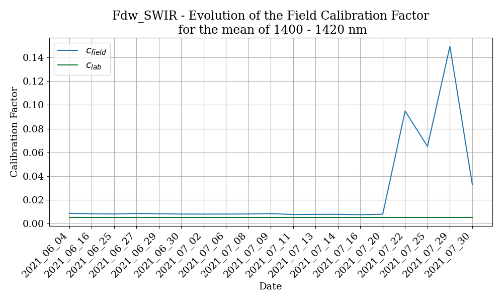
Fig. 1 Evolution of the field calibration factor for ASP06 Fdw SWIR channel.

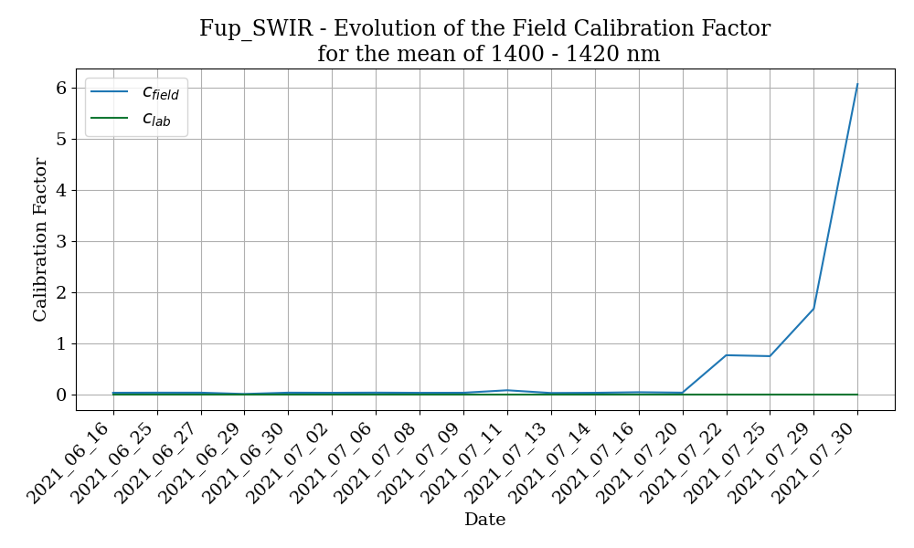
Fig. 2 Evolution of the field calibration factor for ASP06 Fup SWIR channel.

In order to fix this wrong correction of the dark current in the SWIR files the dark current measurements, which were routinely done during the transfer calibrations, can be used. Instead of using the first four measurements the mean of the dark current measurement is used to correct the transfer calibration measurements for the dark current.

After calculating the new field calibration factors with the newly corrected SWIR measurements for all dates after the 22. July it was discovered that the 29. June and the 11. July also show a significantly different field calibration factor for Fup SWIR.

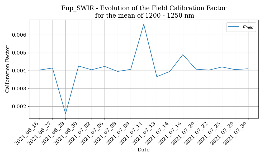
Fig. 3 Evolution of the field calibration factor after new correction of the dark current for 22. - 30. July for ASP06 Fup SWIR channel.

Transfer Calib Fup SWIR 29. June

Looking at the raw measurement from the calibration on 29. June shows that there was a dark current measurement at the beginning, however it seems that the shutter only opened slowly. Usually a jump in the counts should be happening, here only a steady increase in the counts is happening.

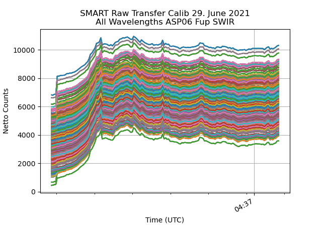
Fig. 4 All wavelengths from the transfer calib measurement of ASP06 Fup SWIR channel.

Using this information the part where the counts gradually increase is cut out from the dark current corrected file before the field calibration factor is calculated with processing.smart_calib_transfer.py . However, this also does not seem to yield a reasonable field calibration factor from that transfer calibration. The most reasonable explanation seems to be that the SWIR spectrometer was unstable during the calibration. In that case it is best to discard this transfer calibration and use another one for the 29. June 2021.

Transfer Calib Fup SWIR 11. July

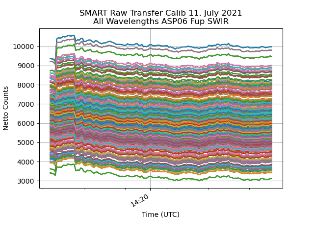
Fig. 5 All wavelengths from the transfer calib measurement of ASP06 Fup SWIR channel.

The first row of the file (2021_07_11_14_19.Fup_SWIR.dat) is deleted as its timestamp lies 12 seconds before the next measurement (see the raw file). Looking at the plot after that first correction was made still shows some weird behaviour. At first the counts decrease during the dark current measurement, then they jump up to a plateau where they increase slightly for a few measurements and then jump down again and slowly decrease until stable conditions are reached roughly at the minute mark (14:20 UTC). Some wavelengths even decrease back to the level of the dark current measurement, hinting at the possibility that the shutter was not working perfectly.

Looking at the corresponding dark current measurement file shows, that the dark current dropped significantly after the first couple of measurements. Thus, to correct the transfer calibration measurement of Fup SWIR only the dark current measurements before the drop in counts at 14:21:03.78 UTC are used to calculate the mean dark current and then correct the calibration measurement by that. The corresponding rows are deleted in the dark current measurement file (everything before 14:21:03.78).

After the dark current correction the rows exhibiting the described weird behaviour are then deleted (everything before before 14:19:50.6).

Transfer Calib Fup SWIR 16. July

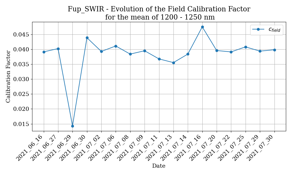
Fig. 6 Evolution of the field calibration factor for ASP06 Fup SWIR channel after the corrections.

After correcting the 11. July the 16. July also shows up as a rather high calibration factor. Looking into the dark current corrected data reveals that the first pixels show only negative values, hinting at a bad dark current measurement at the beginning of the file. Thus, the transfer calibration from the 16. July is also discarded.

Quicklooks generated from the final calibrated files show that the SWIR data is way out of bounds which can be traced back to a very high calibration factor starting on the 21.07.21. Thus, for flights after that date the transfer calibration from 20.07.2021 is used for calibration.

The finally used transfer calibrations can be found in the transfer_calibs dictionary in cirrus_hl.py .

author: Johannes Röttenbacher

smart_process_lab_calib_halo_ac3.py

Correct the lab calibration files for the dark current and merge the minutely files

The calibration was still done with the naming convention of CIRRUS-HL. There are two calibrations available before the campaign both use the VN11 inlet (ASP02) and the optical fiber 22b.

Attention: There was a mixup between VN11 and VN05. Actually VN05 has a nicer cosine response and thus VN05 is used for HALO-(AC)³. However, the calibration was done with VN11 and was repeated after the campaign with VN05.

One calibration was done with VN11 attached to J3 and J4 on ASP06 and the other with VN11 attached to J5 and J6. For HALO-AC3 J3 and J4 were the channels used, because it was written like this in the Einbauanweisung. Thus, only the Fdw measurements are of interest. The Fup measurements are kept for completeness.

author: Johannes Röttenbacher

Final calibration

These scripts are used for the final calibration of the measurement data. They are designed to take care of everything necessary given the correct input files.

cirrus_hl_smart_calibration.py

Complete calibration of the SMART files for the CIRRUS-HL campaign

The dark current corrected SMART measurement files are calibrated and filtered.

• read in dark current corrected files

• calibrate with matching transfer calibration

• correct measurement for cosine dependence of inlet

• add some metadata such as sza and saa

• add stabilization flag for Fdw

• add SMART IMS data

• write to netcdf file (VNIR and SWIR seperate)

• merge VNIR and SWIR data

author: Johannes Röttenbacher

halo_ac3_smart_calibration.py

Complete calibration of the SMART files for the HALO-(AC)³ campaign

The dark current corrected SMART measurement files are calibrated, corrected and filtered.

Steps:

• read in dark current corrected files

• calibrate with matching transfer calibration

• correct measurement for cosine dependence of inlet

• add some metadata such as sza and saa

• add stabilization flag for Fdw

• add SMART IMS data

• write to netcdf file (VNIR and SWIR seperate)

• merge VNIR and SWIR data

• correct attitude for RF18

• add clearsky simulated Fdw

author: Johannes Röttenbacher

BACARDI

BACARDI is a broadband radiometer mounted on the bottom and top of HALO. The data is initially processed by DLR and then Anna Luebke used the scripts provided by André Ehrlich and written by Kevin Wolf to process the data further. During the processing libRadtran simulations of cloud free conditions are done along the flight track of HALO. For details on the BACARDI post processing see BACARDI postprocessing.

Workflow

• download and process the radiosonde data (needs to be done once for each station)

• run libRadtran simulation as explained in BACARDI processing for the whole flight

• run BACARDI postprocessing

Radiosonde data

In order to simulate the clear sky broadband irradiance along the flight path and calculate the direct and diffuse fraction radiosonde data is used as input for libRadtran. The data is downloaded from the University Wyoming website by copying the HTML site into a text file. Data can only be downloaded in monthly chunks. Then an IDL script from Kevin Wolf is used to extract the necessary data for libRadTran. It can be found here: /projekt_agmwend/data/Cirrus_HL/00_Tools/02_Soundings/00_prepare_radiosonde_jr.pro

00_prepare_radiosonde_jr.pro

TODO:

• [ ] Check what radiosonde input is necessary for libRadtran. Simple interpolation yields negative relative humidity at lowest levels. (case: 21.7.21)

Required User Input:

• station name and number (select station closest to flight path)

• quicklook flag

• month

Input:

• monthly radiosonde file

Output:

• daily radiosonde file (12UTC and 00UTC) for libRadtran

Run like this:

# cd into script folder
cd /projekt_agmwend/data/Cirrus_HL/00_Tools/02_soundings
# start idl
idl
# run script
idl> .r 00_prepare_radiosonde_jr

libRadtran simulation

Run libRadtran simulation for solar and terrestrial wavelengths along flight track with specified radiosonde data as input. This is then used in the BACARDI processing. See the section on BACARDI processing for details.

BACARDI postprocessing

Some values are filtered out during the postprocessing. We set an aircraft attitude limit in the processing routine, and if the attitude exceeds this threshold, then the data is filtered out. For example, this would be the case during sharp turns. The threshold also takes the attitude correction factor into account. For CIRRUS-HL, if this factor is below 0.25, then we filter out data where the roll or pitch exceeds 8°. If this factor is above 0.25, then we begin filtering at 5°. For EUREC4A, the limits were not as strict because the SZAs were usually higher. Since this is not the case for the Arctic, something stricter was needed. For more details on other corrections see the processing script. From the processing script:

Solar downward

1. smooth sensor temperature sensor for electronic noise to avoid implications in temperature dependent corrections. - running mean dt=100 sec

2. correct thermophile signal with Temperature dependence of sensor sensitivity (Kipp&Zonen calibration)

3. correct thermal offset due to fast changing temperatures (DLR paramterization using the derivate of the sensor temperature)

4. apply inertness correction of CMP22 sensors (tau_pyrano=1.20, fcut_pyrano=0.6, rm_length_pyrano=0.5)

5. attitude correction (roll_offset=+0.3, pitch_offset=+2.55)

Solar upward

1. smooth sensor temperature sensor for electronic noise to avoid implications in temperature dependent corrections. - running mean dt=100 sec

2. correct thermophile signal with Temperature dependence of sensor sensitivity (Kipp&Zonen calibration)

3. correct thermal offset due to fast changing temperatures (DLR paramterization using the derivate of the sensor temperature)

4. apply inertness correction of CMP22 sensors (tau_pyrano=1.20, fcut_pyrano=0.6, rm_length_pyrano=0.5)

Terrestrial downward

1. smooth sensor temperature sensor for electronic noise to avoid implications in temperature dependent corrections. - running mean dt=100 sec

2. correct thermophile signal with Temperature dependence of sensor sensitivity (Kipp&Zonen calibration)

3. correct thermal offset due to fast changing temperatures (DLR paramterization using the derivate of the sensor temperature)

4. apply inertness correction of CGR4 sensors (tau_pyrano=2.00, fcut_pyrano=0.5, rm_length_pyrano=2.0)

Terretrial upward

1. smooth sensor temperature sensor for electronic noise to avoid implications in temperature dependent corrections. - running mean dt=100 sec

2. correct thermophile signal with Temperature dependence of sensor sensitivity (Kipp&Zonen calibration)

3. correct thermal offset due to fast changing temperatures (DLR paramterization using the derivate of the sensor temperature)

4. apply inertness correction of CGR4 sensors (tau_pyrano=2.00, fcut_pyrano=0.5, rm_length_pyrano=2.0)

00_process_bacardi_V20210928.pro

Required User Input:

• Flight date

• Flight number (Fxx)

Input:

• BACARDI quicklook data from DLR (e.g. QL-CIRRUS-HL_F15_20210715_ADLR_BACARDI_v1.nc)

• simulated broadband downward irradiance from libRadtran

• direct diffuse fraction from libRadtran

Output:

• corrected BACARDI measurement and libRadtran simulations in netCDF file

Run like this:

# cd into script folder
cd /projekt_agmwend/data/Cirrus_HL/00_Tools/01_BACARDI/
# start IDL
idl
# run script
idl> .r 00_process_bacardi_V20210903.pro

BAHAMAS

BAHAMAS records meteorological and location data during the flight. It is mostly used for map plots and information about general flight conditions such as outside temperature, pressure, altitude, speed and so on. It is processed by DLR and there are quicklook files provided during campaign and quality controlled files after the campaign.

libRadtran

libRadtran is a radiative transfer model which can model spectral radiative fluxes.

libRadtran simulations along flight path

The following scripts use the BAHAMAS data to create libRadtran input files to simulate fluxes along the flightpath. The two scripts are meant to allow for flexible settings of the simulation.

BACARDI versions of these scripts are available which replace the old IDL scripts. They are to be used as part of the BACARDI processing. Before publishing BACARDI data, the state of the libRadtran input settings should be saved!

SMART versions of the scripts are also available which run a standard SMART setup for campaign purposes.

TODO:

• [ ] use specific total column ozone concentrations from OMI

  • can be downloaded here: https://disc.gsfc.nasa.gov/datasets/OMTO3G_003/summary?keywords=aura

  • you need an Earth Data account and add the application to your profile

  • checkout the instructions for command line download

• [x] change atmosphere file according to location -> uvspec does this automatically when lat, lon and time are supplied

  • [x] CIRRUS-HL: use midlatitude summer (afglms.dat) or subarctic summer (afglss.dat)

• [x] use ocean or land albedo according to land sea mask

• [x] include solar zenith angle filter

• [ ] use altitude (ground height above sea level) from a surface map, when over land → adjust zout definition accordingly

• [ ] use self-made surface_type_map for simulations in the Arctic

• [ ] use sur_temperature for thermal infrared calculations (input from VELOX)

• BACARDI

• [ ] use surface_type_map for BACARDI simulations

• [ ] use surface temperature according to ERA5 reanalysis for BACARDI simulations

libradtran_write_input_file.py

Create an input files along flight track for libRadtran

Here one can set all options needed in the libRadtran input file. Given the flight and time step, one input file will then be created for every time step with the fitting lat and lon values along the flight track.

Required User Input:

• campaign

• flight (e.g. ‘Flight_202170715a’ or ‘HALO-AC3_20220225_HALO_RF01’)

• time_step (e.g. ‘minutes=1’)

• use_smart_ins flag

• use_dropsonde flag (only available for HALO-(AC)³)

• integrate flag

• input_path, this is where the files will be saved to

Output:

• log file

• input files for libRadtran simulation along flight track

The idea for this script is to generate a dictionary with all options that should be set in the input file. New options can be manually added to the dictionary. The options are linked to the page in the manual where they are described in more detail. Set options to “None” if you don’t want to use them. Variables which start with “_” are for internal use only and will not be used as an option for the input file.

author: Johannes Röttenbacher

libradtran_run_uvspec.py

Run libRadtran simulation (uvspec) for a flight

Given the flight and the path to the uvspec executable, this script calls uvspec for each input file and writes a log and output file. It does so in parallel, checking how many CPUs are available. After that the output files are merged into one data frame and information from the input file is added to write one netCDF file.

The script can be run for one flight or for all flights.

Required User Input:

• campaign

• flight (e.g. “Flight_20210715a” or “HALO-AC3_20220225_HALO_RF01”)

• path to uvspec executable

• wavelength, defines the input folder name which is defined in libradtran_write_input_file.py

• name of netCDF file (optional)

Output:

• out and log file for each simulation

• log file for script

• netCDF file with simulation in- and output

author: Johannes Röttenbacher

BACARDI processing

The following two scripts were used in order to prepare the BACARDI processing. They are superseded by the new python versions of these scripts.

• libradtran_write_input_file_bacardi.py

• libradtran_run_uvspec_bacardi.py

01_dirdiff_BBR_Cirrus_HL_Server_jr.pro

Current settings:

• Albedo from Taylor et al. 1996

• atmosphere file: afglt.dat -> tropical atmosphere

Required User Input:

• Flight date

• sonde date (mmdd)

• sounding station (stationname_stationnumber)

• time interval for modelling (time_step)

Run like this:

# cd into script folder
cd /projekt_agmwend/data/Cirrus_HL/00_Tools/01_BACARDI/
# start IDL
idl
# start logging to a file
idl> journal, 'filename.log'
# run script
idl> .r 01_dirdiff_BBR_Cirrus_HL_Server_jr.pro
# stop logging
idl> journal

03_dirdiff_BBR_Cirrus_HL_Server_ter.pro

Current settings:

• Albedo from Taylor et al. 1996

Required User Input:

• Flight date

• sonde date (mmdd)

• sounding station (stationname_stationnumber)

Run like this:

# cd into script folder
cd /projekt_agmwend/data/Cirrus_HL/00_Tools/01_BACARDI/
# start IDL
idl
# start logging to a file
idl> journal, 'filename.log'
# run script
idl> .r 03_dirdiff_BBR_Cirrus_HL_Server_ter.pro
# stop logging
idl> journal

libradtran_write_input_file_bacardi.py

Create input files for libRadtran simulation to be used in BACARDI processing

This will write all input files for a clearsky broadband libRadtran simulations along the flight path to be compared to BACARDI measurements.

Required User Input:

• flights in a list (optional, if not manually specified all flights will be processed)

• time_step, in what interval should the simulations be done along the flight path?

• solar_flag, write file for simulation of solar or thermal infrared fluxes?

• use_dropsonde flag, only available for HALO-(AC)³

Output:

• log file

• input files for libRadtran simulation along flight track

Run like this:

python libradtran_write_input_file_bacardi.py

Behind some options you find the page number of the manual, where the option is explained in more detail. Set options to “None” if you don’t want to use them. * Variables which start with “_” are for internal use. For HALO-(AC)³ a fixed radiosonde location (Longyearbyen) is used. Uncomment the find_closest_station line for CIRRUS-HL.

author: Johannes Röttenbacher

libradtran_run_uvspec_bacardi.py

Run clearsky broadband libRadtran simulations for comparison with BACARDI measurements.

The input files come from libradtran_write_input_file_bacardi.py.

Required User Input:

• campaign

• flights in a list (optional, if not manually specified all flights will be processed)

• solar_flag, run simulation for solar or for thermal infrared wavelengths?

The script will loop through all files and start simulations for all input files it finds (in parallel for one flight). If the script is called via the command line it creates a log folder in the working directory if necessary and saves a log file to that folder. It also displays a progress bar in the terminal. After it is done with one flight, it will collect information from the input files and merge all output files in a dataframe to which it appends the information from the input files. It converts everything to a netCDF file and writes it to disc with a bunch of metadata included.

Output:

• out and log file for each simulation

• log file for script

• netCDF file with simulation in- and output

Run like this:

python libradtran_run_uvspec_bacardi.py

author: Johannes Röttenbacher

SMART processing

For the calibration of SMART the incoming direct radiation needs to be corrected for the cosine response of the inlet. In order to get the direct fraction of incoming radiation a clearsky simulation is necessary. For this purpose the scripts libradtran_write_input_file_smart.py and libradtran_run_uvspec.py are used. To be able to repeat the simulation the state of the first script which produced the input files for the simulation should not be changed.

libradtran_write_input_file_smart.py

Create an input file for libRadtran to run a SMART clearsky spectral run to calibrate the SMART files.

Required User Input:

• campaign

• flight (e.g. ‘Flight_202170715a’ or ‘HALO-AC3_20220225_HALO_RF01’)

• time_step (e.g. ‘minutes=1’)

• use_smart_ins flag

• use_dropsonde flag (only available for HALO-(AC)³)

Output:

• log file

• input files for libRadtran simulation along flight track

Behind some options you find the page number of the manual, where the option is explained in more detail.

Do not change the options in this file!

This file is part of the SMART calibration and is needed to repeat the calibration. Variables which start with “_” are for internal use only and will not be used as an option for the input file.

author: Johannes Röttenbacher

ecRad

ecRad is the radiation scheme used in the ECMWF’s IFS numerical weather prediction model. For my PhD we are comparing measured radiative fluxes with simulated fluxes along the flight track. For this we run ecRad version 1.5.0 in an offline mode and adjust input parameters. Those experiments are documented in Experiments. Here the general processing with ecRad is described.

Notes

Questions:

• What is the difference between flux_dn_direct_sw and flux_dn_sw in ecrad output? → The second includes diffuse radiation.

• What does gpoint_sw stand for?

General Notes on setting up ecRad

• To avoid a floating point error when running ecrad, run create_practical.sh from the ecrad practical folder in the directory of the ecRad executable once. Somehow the data link is needed to avoid this error. (for version 1.4.1)

• changing the verbosity in the namelist files causes an floating point error (for version 1.4.1)

• decided to use ecRad version 1.5.0 for PhD

Thoughts on the solar zenith angle:

The ultimate goal is to compare irradiances measured by aircraft with the ones simulated by ecRad. A big influence on these irradiances in the Arctic is the solar zenith angle or the cosine thereof. In principle we search for the closest IFS grid point and use this data as input to ecRad. However, for the calculation of the solar zenith angle we should not use the latitude and longitude value of the grid point as these are probably slightly off of the values recorded by the aircraft. This slight offset in position between aircraft and grid point can cause a big difference in solar zenith angle and thus in the simulated irradiances. To avoid additional uncertainty we therefore calculate the solar zenith angle using the latitude and longitude value of the aircraft. As we compare minutely simulations to minutely averages of the measured data, we also take the minutely mean of the BAHAMAS data to get the aircraft’s location.

Folder Structure

├── 0X_ecRad
│   ├── yyyymmdd
│   │   ├── ecrad_input
│   │   ├── ecrad_output
│   │   ├── ecrad_merged
│   │   ├── radiative_properties_vX
│   │   ├── IFS_namelists.nam
│   │   └── ncfiles.nc

Workflow with ecRad

IFS raw output + navigation data from aircraft

→ create ecRad input files which correspond to the columns (+10 surrounding ones) which the aircraft passed during flight

→ run ecrad for aircraft track

SMART/BACARDI measurements during flight + ecRad output files for aircraft track

→ compare upward and downward (spectral/banded) irradiance

1. Download IFS(/CAMS) data for campaign → IFS/CAMS Download

2. Run IFS Preprocessing to convert grib to nc files

3. Run ecrad_read_ifs.py with the options as you want them to be (see script for details)

4. Run ecrad_cams_preprocessing.py to prepare CAMS data

5. Update namelist in the {yyyymmdd} folder with the decorrelation length → choose one value which is representative for the period you want to study

6. Run one of ecrad_write_input_files_vx.py

7. Run ecrad_execute_IFS.sh with options which runs ecRad for each matching file in ecrad_input and then runs the following processing steps

   1. Run ecrad_merge_radiative_properties.py to generate one merged radiative properties file from the single files given by the ecRad simulation

   2. Run ecrad_merge_files.py to generate merged input and output files for and from the ecRad simulation

   3. Run ecrad_processing.py to generate one merged file from input and output files for and from the ecRad simulation with additional variables

In general one can either vary the input to ecRad or the given namelist. For this purpose different input versions can be/were created using modified copies of ecrad_write_input_files.py. They can be found in the experiments folder. An overview of which input versions should be run with which namelist versions can be found in the following table. The version numbers reflect the process in which experiments were thought of or conducted. With version 5 we switched from the interpolated regular lat lon grid (F1280) to the original grid resolution of the IFS which is a octahedral reduced gaussian grid (O1280). The namelists mainly differ in the chosen ice optic parameterization (Fu-IFS, Baran2016, Yi2013) and whether the 3D parameterizations are turned on or not. The output file names of the simulations only differ in the version string (e.g. …_v16.nc) reflecting the namelist version. Thus, many namelists have the same settings but only have different experiment names and the difference comes due to the input. This repetition was chosen to have a better overview of the different combinations of input version and namelist version.

Input version	Namelist version	Short description
1	1, 2, 3.1, 3.2, 4, 5, 6, 7, 12	Original along track data from F1280 IFS output
2	8, 9	Use VarCloud retrieval as iwc and \(r_{eff, ice}\) input along flight track
3	10	Use VarCloud retrieval for below cloud simulation
4	11	Replace q_ice=sum(ciwc, cswc) with q_ice=ciwc
5	13	Set albedo to open ocean (0.06)
5.1	13.1	Set albedo to 0.99
5.2	13.2	Set albedo to BACARDI measurement below cloud
6	15, 18, 19, 22, 24	Along track data from O1280 IFS output (used instead of v1)
6.1	15.1, 18.1, 19.1, 22.1, 24.1, 30, 31, 32	Along track data from O1280 IFS output (used instead of v1) filtered for low clouds
7	16, 20, 26, 27, 28, 33, 34, 35, 36, 37, 38	As v3 but with O1280 IFS output
7.1	16.1, 20.1, 26.1, 27.1, 28.1	As v3 but with O1280 IFS output using re_ice from Sun & Rikus
8	17, 21, 23, 25, 29	As v2 but with O1280 IFS output
9	14	Turn on aerosol and use CAMS data for it

IFS/CAMS Download

To download IFS/CAMS data from the ECMWF servers we got a user account there. For details on how to access and download data there please see the internal Strahlungs Wiki. These are the download scripts used and run on the ECMWF server:

IFS download script: processing.halo_ac3_ifs_download_from_ecmwf.sh

CAMS download script: processing.halo_ac3_cams_downlaod_from_ecmwf.sh (deprecated since 13.10.2023)

The CAMS trace gas climatology was implemented in the ecRad input files on 13.10.2023 (see analysis of impact in Trace gas comparison). Following the usage in the IFS the files provided at https://confluence.ecmwf.int/display/ECRAD were used in ecrad_cams_preprocessing.py.

For the CAMS aerosol climatology another file is available at https://sites.ecmwf.int/data/cams/aerosol_radiation_climatology/. The climatology consists of monthly means on a 3°x3° grid with 60 levels and gives the aerosol concentration as a layer integrated mass (\(m_{\text{int}}\)) in \(\text{kg}\,\text{m}^{-2}\). The file also gives the pressure at the base of each layer and the pressure difference between the top and the base of each layer:

\[\Delta p = p(n+1) - p(n), n = (1, ..., 60).\]

The pressure can be used to interpolate the data to the 137 full pressure levels of the IFS. Further, the aerosol mass mixing ratio in \(\text{kg}\,\text{kg}^{-1}\) can be calculated by dividing the layer integrated mass by the total layer integrated mass:

\[\text{MMR} = \frac{m_{\text{int}}}{m_{\text{layer}}} = \frac{m_{\text{int}}}{\Delta p / g},\]

with \(\Delta p\) being the pressure difference between the model half levels and \(g = 9.80665\,\text{m}\,\text{s}^{-2}\) the gravitational acceleration.

Another option would be to download the monthly mean CAMS files from the Copernicus Atmospheric Data Store (ADS) and use these files. The script processing.download_cams_data.py downloads the CAMS aerosol and trace gas climatology and saves them to seperate files.

IFS Preprocessing

IFS data comes in grib format. To convert it to netcdf and rename the parameters according to the ECMWF codes run

cdo --eccodes -f nc copy infile.grb outfile.nc

on each file. Or run the python script processing.ecrad_preprocessing.py (currently only working for IFS files):

ecrad_preprocessing.py

author: Johannes Röttenbacher

created: 18.09.2023

Convert raw IFS surface and multilevel file from grib to netCDF. Use cdo to decode grib file and save it to netCDF. Will not overwrite existing files.

Required User Input:

• date (e.g. 20220313, all)

If date=all runs for all flights.

Run like this:

python processing/ecrad_preprocessing.py date=all

CAMS files (deprecated since 13.10.2023)

Warning

Deprecated since 13.10.2023 This is not needed since there is a monthly mean product available on the ADS!

We want to get yearly monthly means from the CAMS reanalysis. For this we download 3-hourly data and preprocess it on the ECMWF server to avoid downloading a huge amount of data.

CAMS preprocessing script: processing.halo_ac3_preprocess_cams_data_on_ecmwf.py

The CAMS monthly files are not so big. Thus, you can merge them into one big file and run the above command only on one file. The merging and conversion to netCDF will take a while though. The download script for CAMS data generates yearly folders for better structure in case more than two months are downloaded. You can move all files into one folder by calling the following command in the CAMS folder and then merge the files with cdo:

mv --target-directory=. 20*/20*.grb
cdo mergetime 20*.grb cams_ml_halo_ac3.grb

ecrad_read_ifs.py

author: Hanno Müller, Johannes Röttenbacher

created: 22-09-2022

Data extraction from IFS along the flight track

TODO:

• [x] more precise read in of navigation data

• [x] test if it is necessary to generate one file per time step → it is

• [ ] Include an option to interpolate in space

• [x] check why file 1919-1925 + 6136-6180 + 7184-7194 cause a floating-point exception when processed with ecrad (discovered 2021-04-26) -> probably has to do the way ecrad is called (see execute_IFS.sh)

Input:

• IFS model level (ml) file

• IFS surface (sfc) file

• SMART horidata with flight track or BAHAMAS file

• Ozone sonde (optional)

Required User Input:

Can be passed via the command line (except step).

• campaign (‘halo-ac3’ or ‘cirrus-hl’)

• key (e.g. RF17)

• init_time (00, 12 or yesterday)

• flight (e.g. ‘Flight_20210629a’ or ‘HALO-AC3_20220412_HALO_RF18’)

• aircraft (‘halo’)

• use_bahamas, whether to use BAHAMAS or the SMART INS for navigation data (True/False)

• grid (O1280 or None), which grid the IFS data is on

• step, one can choose the time resolution on which to interpolate the IFS data on (e.g. ‘1Min’)

Output:

• processed IFS file for input to ecrad_write_input_files_vx.py

• decorrelation length for ecRad namelist file → manually change that in the namelist file

ecrad_cams_preprocessing.py

author: Johannes Röttenbacher

created: 10.10.2023

Select closest points of CAMS global reanalysis and global greenhouse gas reanalysis data to flight track. Read in CAMS from different sources (ADS, Copernicus Knowledge Base (47r1)). The Copernicus Atmospheric Data Store provides the monthly means of trace gase concentrations and aerosol concentrations. They are the basis for the files available via the Copernicus Knowledge Base. However, these files have been processed a bit before their use in the IFS. See IFS/CAMS Download for more details and the links to the files.

Required User Input:

• source (47r1, ADS)

• year (2020, 2019)

• date (20220411)

Input:

• monthly mean CAMS data

• greenhouse gas time series (needed if source is ‘47r1’)

Output:

• trace gas and aerosol monthly climatology interpolated to flight day along flight track

ecrad_write_input_files_vx.py

author: Johannes Röttenbacher

created: 22-09-2022

Deprecated since version 0.7.0: Use experiments.ecrad_write_input_files_vx.py instead!

Use a processed IFS output file and generate one ecRad input file for each time step. Can be called from the command line with the following key=values pairs:

• t_interp (default: False)

• date (default: ‘20220411’)

• init_time (default: ‘00’)

• flight (default: ‘HALO-AC3_20220411_HALO_RF17’)

• aircraft (default: ‘halo’)

• campaign (default: ‘halo-ac3’)

Output:

• well documented ecRad input file in netCDF format for each time step

ecrad_execute_IFS.sh

This script loops through all input files and runs ecrad with the setup given in IFS_namelist_jr_{date}_{version}.nam.

Attention (version 1.4.1): ecRad has to be run without full paths for the input and output nc file. Only the namelist has to be given with its full path. The namelist has to be in the same folder as the input files and the output files have to be written in the same folder.

The date defines the input path which is generally /projekt_agmwend/data/{campaign}/{ecrad_folder}/ecrad_input/yyyymmdd/. It then writes the output to the given output path, one output file per input file. The radiative_properties.nc file which is optionally generated in each run depending on the namelist is renamed and moved to a separate folder to avoid overwriting the file.

Input:

• ecrad input files

• IFS namelist

Required User Input:

• -t: use the time interpolated data (default: False)

• -d yyyymmdd: give the date to be processed

• -v v1: select which namelist version (experimental setup) to use (see ecRad Namelists and Experiments for details on version)

• -i v1: select which input version to use

Output:

• ecrad output files

• radiative_properties.nc moved to a separate folder and renamed according to input file (optional)

Run like this:

This will write all output to the console and to the specified file.

. ./ecrad_execute_IFS.sh [-t] [-d yyyymmdd] [-v v1] [-i v1] 2>&1 | tee ./log/today_ecrad_yyyymmdd.log

ecrad_execute_IFS_single.sh

As above but runs only one file which has to be defined in the script.

ecrad_merge_radiative_properties.py

author: Johannes Röttenbacher

created: 21-04-2023

Merge radiative properties nc files created by ecRad

This script takes all radiative property files created by ecRad as additional output and merges them. Each radiative property file has its time stamp in the file name (seconds of day) and can potentially have only a few columns in it. How many columns are saved in one radiative property file depends on the n_blocksize namelist option.

It can be run via the command line and accepts several keyword arguments.

Run like this:

python ecrad_merge_radiative_properties.py base_dir="./data_jr" date=yyyymmdd version=v1

This would merge all radiative property files which can be found in {base_dir}/{date}/radiative_properties_{version}/.

User Input:

• date (yyyymmdd)

• version (vx, default:v1)

• base_dir (directory, default: ecrad directory for halo-ac3 campaign)

Output:

• log file

• intermediate merged files in {base_dir}/radiative_properties_merged/

• final merged file: {base_dir}/radiative_properties_merged_{yyyymmdd}_{version}.nc

ecrad_merge_files.py

Bundle postprocessing steps for ecRad input and output files

This script takes all in- and outfiles for and from ecRad and merges them together on a given time axis which is constructed from the file names. That should rapidly increase further work with ecRad data. It merges stepwise to reduce IO. In a selectable step the merged input and output files can also be merged.

It can be run via the command line and accepts several keyword arguments.

Run like this:

python ecrad_merge_files.py io_flag=input t_interp=False base_dir="./data_jr" date=yyyymmdd merge_io=T

This would merge all ecrad input files which are not time interpolated and can be found in {base_dir}/{date}/ecrad_input/. After that the script would try to merge the merged in- and outfiles into one file. If only merge_io is given only this would happen:

# merge merged in- and outfiles
python ecrad_merge_files.py merge_io=T date=yyyymmdd

Usually one would first call it to merge all input files and then a second time to merge all output files and merge them with the merged input files.

User Input:

• io_flag (input, output or None, default: None)

• date (yyyymmdd)

• version (vx, default:v1)

• t_interp (True or False, default: False)

• base_dir (directory, default: ecrad directory for halo-ac3 campaign)

• merge_io (T, optional)

Output:

• log file

• intermediate merged files in {base_dir}/ecrad_merged/

• final merged file: {base_dir}/ecrad_merged_(input/output)_{yyyymmdd}(_inp).nc

• possibly {base_dir}/ecrad_merged_inout_{yyyymmdd}(_inp).nc

author: Johannes Röttenbacher

ecrad_processing.py

author: Johannes Röttenbacher

created: 20.04.2023

Bundle calculation of additional variables for ecRad input and output files

This script calculates a few additional variables which are often needed when working with ecRad in- and output data. After that it also saves a file containing the mean over all columns.

It can be run via the command line and accepts several keyword arguments.

Run like this:

python ecrad_processing.py date=yyyymmdd base_dir="./data_jr" iv=v1 ov=v1

This would merge the version 1 merged input files with the version 1 merged output files which can be found in {base_dir}/{date} and add some variables.

User Input:

• date (yyyymmdd)

• base_dir (directory, default: ecrad directory for halo-ac3 campaign)

• iv (vx, default:v1) input file version

• ov (vx, default:v1) output file version

Output:

• log file

• merged input and output file: {base_dir}/ecrad_merged_inout_{yyyymmdd}_{ov}.nc

GoPro Time Lapse quicklooks

During the flight a GoPro was attached to one of the windows of HALO. Using the time-lapse function a picture was taken every 5 seconds. Together with BAHAMAS position data (and SMART spectra measurements) a time-lapse video is created. The GoPro was set to UTC time but cannot be synchronized to BAHAMAS. Thus, a foto of the BAHAMAS time server is taken at the start of each recording to determine the offset of the camera from the fotos metadata.

During CIRRUS-HL the camera reset its internal time to local time, so the metadata for some flights had to be corrected for that as well. See the README.md in the CIRRUS-HL GoPro folder for details. A list which tracks the processing status can be found there. For HALO-(AC)³ this table is part of the processing_diary.md which can be found in the upper level folder HALO-AC3.

gopro_copy_files_to_disk.py

Copy all files from the GoPro SD Card into one folder

Required User Input:

• date

• src, source directory

• dst_dir, destination directory

author: Johannes Roettenbacher

gopro_add_timestamp_to_picture.py

Add a timestamp to a GoPro picture and correct the metadata

Run on Linux!

This script reads out the DateTimeOriginal metadata tag of each file and corrects it for the Local Time to UTC and BAHAMAS offset if necessary. It overwrites the original metadata tag and places a time stamp to the right bottom of the file. One can test the time correction by replacing path with file in run() (line 66).

Required User Input:

• campaign

• flight

• correct_time flag

• filename for a test file

• LT_to_UTC flag (CIRRUS-HL only)

• path with all GoPro pictures

Output:

• overwrites metadata in original file with UTC time from BAHAMAS

• adds a time stamp to the right bottom of the original file

author: Johannes Röttenbacher

gopro_write_timestamps.py

Read out timestamps from GoPro images and write to a text file

Run on Linux!

Reads the metadata time stamps and saves them together with the picture number in a csv file.

Required User Input:

• campaign

• flight

Output:

• txt file with exiftool output

• csv file with datetime from picture metadata and picture number

Steps:

• use exiftool to get timestamps of GoPro images

• write the output to a textfile

• read the textfile line by line and extract the picture number and datetime

• convert to pd.datetime and correct for the time offset to BAHAMAS

• create DataFrame and save to csv

author: Johannes Röttenbacher

gopro_plot_maps.py

Plotting script for map plots to be used in time-lapse videos of GoPro

Required User Input:

• campaign

• flight

• use_smart_ins flag

• second airport to add to map

• csv file with time stamp and GoPro picture number (output from gopro_write_timestamps.py)

• BAHAMAS nc file

Output:

• csv file with selected GoPro picture numbers and timestamps which are used for the time-lapse video

• map for each GoPro picture

Reads in the BAHAMAS latitude and longitude data and selects only the time steps which correspond with a GoPro picture. In the plot_props dictionary the map layout properties for each flight are defined. For testing the first four lines of the last cell can be uncommented and the Parallel call can be commented. It makes sense to run this script on the server to utilize more cores and increase processing speed.

author: Johannes Röttenbacher

gopro_add_map_to_picture.py

Add the bahamas map to a picture

Run on Linux!

Required User Input:

• campaign

• flight

• maps

• map numbers from csv file (output of gopro_plot_maps.py)

Output: new GoPro picture with map in the upper right corner and timestamp in the lower right corner

Saves to a new directory!

Adds the BAHAMAS plot onto the GoPro picture but only for pictures, which were taken in flight, according to a csv file. Saves those pictures in a new folder: {flight}_map.

author: Johannes Roettenbacher

gopro_make_video_from_pictures.sh

Uses ffmpeg to create a stop-motion video of the GoPro pictures.

Run on Linux!

Required User Input:

• flight

• base directory of GoPro images

• framerate [12, 24]

• start_number, number in filename of first picture in folder

Output: video (slow or fast) of flight from GoPro pictures

Other

Instrument independent processing scripts.

halo_calculate_attitude_correction.py

Calculate attitude correction for BACARDI and for SMART from BAHAMAS data

Rationale

SMART is stabilized, however the stabilization does not work perfectly all the time. By calculating the attitude correction for an unstabilized case and applying this backwards on a libRadtran simulation can tell us more about, how well the stabilization worked and the impact of its imperfection. The attitude angles have to be interpolated onto the libRadtran time steps before the correction can be calculated. The attitude correction can also be used for the BACARDI data.

Save the attitude correction in the respective time resolutions for BACARDI, SMART and libRadtran.

author: Johannes Röttenbacher

ifs_calculate_along_track_stats.py

Calculate statistics from the ECMWF IFS output along the flight track

Using the BAHAMAS down sampled data (0.5Hz) and a defined circle around the closest IFS grid point to the aircraft location, statistics from the IFS output are calculated and saved to new netCDF files for use in the case studies.

Input:

• IFS data as returned by read_ifs.py

• BAHAMAS data

• ecRad output data

Output:

NetCDF files in the IFS input directory with the statistics.

TODO: Add option to vary amount of surrounding grid cells

author: Johannes Röttenbacher