Experiments

Here different model setups and experiments are documented and discussed. A lot of knobs can be turned in models. This chapter is meant to track the different model setup used and their results.

ecRad Namelists and Experiments

Namelists can be found in the corresponding date folder in the ecrad folder for each campaign (see config.toml).

• IFS_namelist.nam: Namelist as used by Kevin

• IFS_namelist_jr.nam: Adjusted namelist for first runs by Johannes

• IFS_namelist_v2.nam: Namelist with spectral short wave albedo enabled

• IFS_namelist_hanno_org.nam: Used by Hanno

CIRRUS-HL 2021-06-29

• IFS_namelist_jr_20210629a_v1.nam: for flight 20210629a with Fu-IFS ice model

• IFS_namelist_jr_20210629a_v2.nam: for flight 20210629a with Baran2017 ice model (deprecated)

• IFS_namelist_jr_20210629a_v3.nam: for flight 20210629a with Baran2016 ice model

• IFS_namelist_jr_20210629a_v4.nam: for flight 20210629a with Yi2013 ice model

HALO-(AC)³ 2022-04-11

• vxx.1: uses input version vx.1 instead of vx

• v6.1: with low clouds filtered

• v6.2: with low clouds filtered and cosine dependence of ice effective radius removed

• v7.1: instead of using the VarCloud retrieved re_ice use Sun & Rikus to calculate it from the VarCloud IWC

• v7.2: instead of using the VarCloud retrieved re_ice use Sun & Rikus to calculate it from the VarCloud IWC and remove cosine dependence of minimum re_ice

Table 1 ecRad version overview

Version	Input Version	Ice Optics Parameterization	3D Parameterization	Aerosol Optics
v1	v1	Fu-IFS	Off	Off
v3.1	v1	Fu-IFS	Off	Off
v3.2	v1	Fu-IFS	Off	Off
v4	v1	Yi2013	Off	Off
v5	v1	Fu-IFS	On	Off
v6	v1	Baran2016	On	Off
v7	v1	Baran2016	Off	Off
v8	v2	Fu-IFS	Off	Off
v9	v2	Baran2016	Off	Off
v10	v3	Fu-IFS	Off	Off
v11	v4	Fu-IFS	Off	Off
v12	v1	Fu-IFS	Off	Off
v13	v5	Fu-IFS	Off	Off
v13.1	v5	Fu-IFS	Off	Off
v13.2	v5	Fu-IFS	Off	Off
v14	v9	Fu-IFS	Off	Off
v15	v6	Fu-IFS	Off	Off
v16	v7	Fu-IFS	Off	Off
v17	v8	Fu-IFS	Off	Off
v18	v6	Baran2016	Off	Off
v19	v6	Yi2013	Off	Off
v20	v7	Baran2016	Off	Off
v21	v8	Baran2016	Off	Off
v22	v6	Fu-IFS	On	Off
v23	v8	Fu-IFS	On	Off
v24	v6	Baran2016	On	Off
v25	v8	Baran2016	On	Off
v26	v7	Fu-IFS	On	Off
v27	v7	Baran2016	On	Off
v28	v7	Yi2013	Off	Off
v29	v8	Yi2013	Off	Off
v30	v6	Fu-IFS	Off	On
v31	v6	Yi2013	Off	On
v32	v6	Baran2016	Off	On
v33	v7	Fu-IFS	Off	On
v34	v7	Yi2013	Off	On
v35	v7	Baran2016	Off	On
v36	v7	Fu-IFS	Off	Off
v37	v7	Yi2013	Off	Off
v38	v7	Baran2016	Off	Off
v39	v6	Fu-IFS	Off	Off
v40	v6	Yi2013	Off	Off
v41	v7	Fu-IFS	Off	Off
v42	v7	Yi2013	Off	Off

Input version	Namelist version	Short description
1	1, 2, 3.1, 3.2, 4, 5, 6, 7, 12	Original along track data from F1280 IFS output
2	8, 9	Use VarCloud retrieval as iwc and \(r_{eff, ice}\) input along flight track
3	10	Use VarCloud retrieval for below cloud simulation
4	11	Replace q_ice=sum(ciwc, cswc) with q_ice=ciwc
5	13	Set albedo to open ocean (0.06)
5.1	13.1	Set albedo to 0.99
5.2	13.2	Set albedo to BACARDI measurement below cloud
6	15, 18, 19, 22, 24	Along track data from O1280 IFS output (used instead of v1)
6.1	15.1, 18.1, 19.1, 22.1, 24.1, 30.1, 31.1, 32.1	As above but filtered for low clouds
6.2	39.2, 40.2	As above but with latitude set to 0 to remove cosine dependence of the ice effective radius
7	16, 20, 26, 27, 28, 33, 34, 35, 36, 37, 38	As v3 but with O1280 IFS output
7.1	16.1, 20.1, 26.1, 27.1, 28.1	As above but using re_ice from Sun & Rikus
7.2	41.2, 42.2	As above but with latitude set to 0 to remove cosine dependence of the ice effective radius
8	17, 21, 23, 25, 29	As v2 but with O1280 IFS output
9	14	Turn on aerosol and use CAMS data for it
10	43.1	Use specific humidity from dropsondes

• IFS_namelist_jr_20220411_v1.nam: for RF17 with Fu-IFS ice model

• IFS_namelist_jr_20220411_v2.nam: for RF17 with Baran2017 ice model (deprecated)

• IFS_namelist_jr_20220411_v3.1.nam: for RF17 with Fu-IFS ice model and overlap_decorr_length = 1028 m

• IFS_namelist_jr_20220411_v3.2.nam: for RF17 with Fu-IFS ice model and overlap_decorr_length = 450 m

• IFS_namelist_jr_20220411_v4.nam: for RF17 with Yi2013 ice model

• IFS_namelist_jr_20220411_v5.nam: for RF17 with Fu-IFS ice model and 3D parameterizations enabled

• IFS_namelist_jr_20220411_v6.nam: for RF17 with Baran2016 ice model and 3D parameterizations enabled

• IFS_namelist_jr_20220411_v7.nam: for RF17 with Baran2016 ice model

• IFS_namelist_jr_20220411_v8.nam: for RF17 with Fu-IFS ice model using VarCloud retrieval for q_ice and re_ice input (input version v2)

• IFS_namelist_jr_20220411_v9.nam: for RF17 with Baran2016 ice model using VarCloud retrieval for q_ice and re_ice input (input version v2)

• IFS_namelist_jr_20220411_v10.nam: for RF17 with Fu-IFS ice model using VarCloud retrieval for q_ice and re_ice for the below cloud section as well (input version v3)

• IFS_namelist_jr_20220411_v11.nam: for RF17 with Fu-IFS ice model using ciwc as q_ice instead of sum(ciwc, cswc) (input version v4)

• IFS_namelist_jr_20220411_v12.nam: for RF17 with Fu-IFS ice model using general cloud optics

• IFS_namelist_jr_20220411_v13.nam: for RF17 with Fu-IFS ice model setting albedo to open ocean (input version v5)

• IFS_namelist_jr_20220411_v13.1.nam: for RF17 with Fu-IFS ice model setting albedo to 0.99 (input version v5.1)

• IFS_namelist_jr_20220411_v13.2.nam: for RF17 with Fu-IFS ice model setting albedo to BACARDI measurements belwo cloud (input version v5.2)

• IFS_namelist_jr_20220411_v14.nam: for RF17 with Fu-IFS ice model including aerosol in run (TBD, input version v9)

• IFS_namelist_jr_20220411_v15.nam: for RF17 with Fu-IFS ice model using O1280 IFS data (input version v6)

• IFS_namelist_jr_20220411_v16.nam: for RF17 with Fu-IFS ice model using O1280 IFS data and VarCloud retrieval for q_ice and re_ice input for the below cloud section (input version v7)

• IFS_namelist_jr_20220411_v17.nam: for RF17 with Fu-IFS ice model using O1280 IFS data and VarCloud retrieval for q_ice and re_ice input (input version v8)

• IFS_namelist_jr_20220411_v18.nam: for RF17 with Baran2016 ice model using O1280 IFS data (input version v6)

• IFS_namelist_jr_20220411_v19.nam: for RF17 with Yi2013 ice model using O1280 IFS data (input version v6)

• IFS_namelist_jr_20220411_v20.nam: for RF17 with Baran2016 ice model using O1280 IFS data and the VarCloud retrieval for q_ice and re_ice input for the below cloud section (input version v7)

• IFS_namelist_jr_20220411_v21.nam: for RF17 with Baran2016 ice model using O1280 IFS data and the VarCloud retrieval for q_ice and re_ice input (input version v8)

• IFS_namelist_jr_20220411_v22.nam: for RF17 with Fu-IFS ice model using O1280 IFS data and 3D parameterizations enabled (input version v6)

• IFS_namelist_jr_20220411_v23.nam: for RF17 with Fu-IFS ice model using O1280 IFS data and VarCloud retrieval for q_ice and re_ice input and 3D parameterizations enabled (input version v8)

• IFS_namelist_jr_20220411_v24.nam: for RF17 with Baran2016 ice model using O1280 IFS and 3D parameterizations enabled (input version v6)

• IFS_namelist_jr_20220411_v25.nam: for RF17 with Baran2016 ice model using O1280 IFS and VarCloud retrieval for q_ice and re_ice input and 3D parameterizations enabled (input version v8)

• IFS_namelist_jr_20220411_v26.nam: for RF17 with Fu-IFS ice model using O1280 IFS data and VarCloud retrieval for q_ice and re_ice input below cloud and 3D parameterizations enabled (input version v7)

• IFS_namelist_jr_20220411_v27.nam: for RF17 with Baran2016 ice model using O1280 IFS and VarCloud retrieval for q_ice and re_ice input below cloud and 3D parameterizations enabled (input version v7)

• IFS_namelist_jr_20220411_v28.nam: for RF17 with Yi2013 ice model using O1280 IFS and VarCloud retrieval for q_ice and re_ice input below cloud (input version v7)

• IFS_namelist_jr_20220411_v29.nam: for RF17 with Yi2013 ice model using O1280 IFS and VarCloud retrieval for q_ice and re_ice input (input version v8)

• IFS_namelist_jr_20220411_v30.nam: for RF17 with Fu-IFS ice model using O1280 IFS and aerosols turned on (input version v6.1)

• IFS_namelist_jr_20220411_v31.nam: for RF17 with Yi2013 ice model using O1280 IFS and aerosols turned on (input version v6.1)

• IFS_namelist_jr_20220411_v32.nam: for RF17 with Baran2016 ice model using O1280 IFS and aerosols turned on (input version v6.1)

• IFS_namelist_jr_20220411_v33.nam: for RF17 with Fu-IFS ice model using O1280 IFS, VarCloud retrieval for q_ice and re_ice input and aerosols turned on (input version v7)

• IFS_namelist_jr_20220411_v34.nam: for RF17 with Yi2013 ice model using O1280 IFS, VarCloud retrieval for q_ice and re_ice input and aerosols turned on (input version v7)

• IFS_namelist_jr_20220411_v35.nam: for RF17 with Baran2016 ice model using O1280 IFS, VarCloud retrieval for q_ice and re_ice input and aerosols turned on (input version v7)

• IFS_namelist_jr_20220411_v36.nam: for RF17 with Fu-IFS ice model using O1280 IFS, VarCloud retrieval for q_ice and re_ice input below cloud, turned fractional standard deviation to 0 (measure for inhomogeneity) (input version v7)

• IFS_namelist_jr_20220411_v37.nam: for RF17 with Yi2013 ice model using O1280 IFS, VarCloud retrieval for q_ice and re_ice input below cloud, turned fractional standard deviation to 0 (measure for inhomogeneity) (input version v7)

• IFS_namelist_jr_20220411_v38.nam: for RF17 with Baran2016 ice model using O1280 IFS, VarCloud retrieval for q_ice and re_ice input below cloud, turned fractional standard deviation to 0 (measure for inhomogeneity) (input version v7)

• IFS_namelist_jr_20220411_v39.2.nam: for RF17 with Fu-IFS ice model using O1280 IFS, turned of cosine dependence of minimum re_ice (input version v6.2)

• IFS_namelist_jr_20220411_v40.2.nam: for RF17 with Yi2013 ice model using O1280 IFS, turned of cosine dependence of minimum re_ice (input version v6.2)

• IFS_namelist_jr_20220411_v41.2.nam: for RF17 with Fu-IFS ice model using O1280 IFS and VarCloud retrieval for q_ice input for the below cloud section, re_ice is calculated with Sun & Rikus from VarCloud IWC but with turned of cosine dependence of minimum re_ice (input version v7.2)

• IFS_namelist_jr_20220411_v42.2.nam: for RF17 with Yi2013 ice model using O1280 IFS and VarCloud retrieval for q_ice input for the below cloud section, re_ice is calculated with Sun & Rikus from VarCloud IWC but with turned of cosine dependence of minimum re_ice (input version v7.2)

• IFS_namelist_jr_20220411_v43.1.nam: for RF17 with Fu-IFS ice model using O1280 IFS data (input version v10)

HALO-(AC)³ 2022-04-12

• vxx.1: uses input version vx.1 instead of vx

• v6.1: with low clouds filtered

• v7.1: instead of using the VarCloud retrieved re_ice use Sun & Rikus to calculate it

• IFS_namelist_jr_20220412_v1.nam: for RF18 with Fu-IFS ice model

• IFS_namelist_jr_20220412_v8.nam: for RF18 with Fu-IFS ice model using VarCloud retrieval for q_ice and re_ice input

• IFS_namelist_jr_20220412_v11.nam: for RF18 with Fu-IFS ice model using ciwc as q_ice instead of sum(ciwc, cswc)

• IFS_namelist_jr_20220412_v15.nam: for RF18 with Fu-IFS ice model using O1280 IFS data (input version v6)

• IFS_namelist_jr_20220412_v16.nam: for RF18 with Fu-IFS ice model using O1280 IFS data and VarCloud retrieval for q_ice and re_ice input for the below cloud section (input version v7)

• IFS_namelist_jr_20220412_v17.nam: for RF18 with Fu-IFS ice model using O1280 IFS data and VarCloud retrieval for q_ice and re_ice input (input version v8)

• IFS_namelist_jr_20220412_v18.nam: for RF18 with Baran2016 ice model using O1280 IFS data (input version v6)

• IFS_namelist_jr_20220412_v19.nam: for RF18 with Yi2013 ice model using O1280 IFS data (input version v6)

• IFS_namelist_jr_20220412_v20.nam: for RF18 with Baran2016 ice model using O1280 IFS data and the VarCloud retrieval for q_ice and re_ice input for the below cloud section (input version v7)

• IFS_namelist_jr_20220412_v21.nam: for RF18 with Baran2016 ice model using O1280 IFS data and the VarCloud retrieval for q_ice and re_ice input (input version v8)

• IFS_namelist_jr_20220412_v22.nam: for RF18 with Fu-IFS ice model using O1280 IFS data and 3D parameterizations enabled (input version v6)

• IFS_namelist_jr_20220412_v23.nam: for RF18 with Fu-IFS ice model using O1280 IFS data and VarCloud retrieval for q_ice and re_ice input and 3D parameterizations enabled (input version v8)

• IFS_namelist_jr_20220412_v24.nam: for RF18 with Baran2016 ice model using O1280 IFS and 3D parameterizations enabled (input version v6)

• IFS_namelist_jr_20220412_v25.nam: for RF18 with Baran2016 ice model using O1280 IFS and VarCloud retrieval for q_ice and re_ice input and 3D parameterizations enabled (input version v8)

• IFS_namelist_jr_20220412_v26.nam: for RF18 with Fu-IFS ice model using O1280 IFS data and VarCloud retrieval for q_ice and re_ice input below cloud and 3D parameterizations enabled (input version v7)

• IFS_namelist_jr_20220412_v27.nam: for RF18 with Baran2016 ice model using O1280 IFS and VarCloud retrieval for q_ice and re_ice input below cloud and 3D parameterizations enabled (input version v7)

• IFS_namelist_jr_20220412_v28.nam: for RF18 with Yi2013 ice model using O1280 IFS and VarCloud retrieval for q_ice and re_ice input below cloud (input version v7)

• IFS_namelist_jr_20220412_v29.nam: for RF18 with Yi2013 ice model using O1280 IFS and VarCloud retrieval for q_ice and re_ice input (input version v8)

• IFS_namelist_jr_20220412_v30.nam: for RF18 with Fu-IFS ice model using O1280 IFS and aerosols turned on (input version v6.1)

• IFS_namelist_jr_20220412_v31.nam: for RF18 with Yi2013 ice model using O1280 IFS and aerosols turned on (input version v6.1)

• IFS_namelist_jr_20220412_v32.nam: for RF18 with Baran2016 ice model using O1280 IFS and aerosols turned on (input version v6.1)

• IFS_namelist_jr_20220412_v33.nam: for RF18 with Fu-IFS ice model using O1280 IFS, VarCloud retrieval for q_ice and re_ice input and aerosols turned on (input version v7)

• IFS_namelist_jr_20220412_v34.nam: for RF18 with Yi2013 ice model using O1280 IFS, VarCloud retrieval for q_ice and re_ice input and aerosols turned on (input version v7)

• IFS_namelist_jr_20220412_v35.nam: for RF18 with Baran2016 ice model using O1280 IFS, VarCloud retrieval for q_ice and re_ice input and aerosols turned on (input version v7)

• IFS_namelist_jr_20220412_v36.nam: for RF18 with Fu-IFS ice model using O1280 IFS, VarCloud retrieval for q_ice and re_ice input below cloud, turned fractional standard deviation to 0 (measure for inhomogeneity) (input version v7)

• IFS_namelist_jr_20220412_v37.nam: for RF18 with Yi2013 ice model using O1280 IFS, VarCloud retrieval for q_ice and re_ice input below cloud, turned fractional standard deviation to 0 (measure for inhomogeneity) (input version v7)

• IFS_namelist_jr_20220412_v38.nam: for RF18 with Baran2016 ice model using O1280 IFS, VarCloud retrieval for q_ice and re_ice input below cloud, turned fractional standard deviation to 0 (measure for inhomogeneity) (input version v7)

• IFS_namelist_jr_20220412_v39.2.nam: for RF18 with Fu-IFS ice model using O1280 IFS, turned of cosine dependence of minimum re_ice (input version v6.2)

• IFS_namelist_jr_20220412_v40.2.nam: for RF18 with Yi2013 ice model using O1280 IFS, turned of cosine dependence of minimum re_ice (input version v6.2)

• IFS_namelist_jr_20220412_v41.2.nam: for RF18 with Fu-IFS ice model using O1280 IFS and VarCloud retrieval for q_ice input for the below cloud section, re_ice is calculated with Sun & Rikus from VarCloud IWC but with turned of cosine dependence of minimum re_ice (input version v7.2)

• IFS_namelist_jr_20220412_v42.2.nam: for RF18 with Yi2013 ice model using O1280 IFS and VarCloud retrieval for q_ice input for the below cloud section, re_ice is calculated with Sun & Rikus from VarCloud IWC but with turned of cosine dependence of minimum re_ice (input version v7.2)

• IFS_namelist_jr_20220412_v43.1.nam: for RF18 with Fu-IFS ice model using O1280 IFS data (input version v10)

Overlap decorrelation length experiment

Script: ecrad_experiment_v3_x.py

Evaluation of the influence of the overlap decorrelation length parameter

Problem: The parameterization of cloud overlap in ecRad, the so-called cloud overlap decorrelation length, can only be given in the Fortran namelist but changes with latitude. It should be avoided to create a new namelist for each time step of the along track simulation.

Here the influence of the overlap decorrelation length on the RF17 case study of single layer Arctic cirrus is investigated. Two simulations are performed using the maximum and minimum calculated overlap decorrelation length after Shonk et al. [2010] along the flight path. See /projekt_agmwend/data/HALO-AC3/09_IFS_ECMWF/20220411/20220411_decorrelation_length.csv for values in km. Input file from dropsonde location at 11:01 UTC: ecrad_input_standard_39660.0_sod_v1.nc

• IFS_namelist_jr_20220411_v3.1.nam: for flight HALO-AC3_20220411_HALO_RF17 with Fu-IFS ice model and overlap_decorr_length = 1028 m

• IFS_namelist_jr_20220411_v3.2.nam: for flight HALO-AC3_20220411_HALO_RF17 with Fu-IFS ice model and overlap_decorr_length = 450 m

Results

The actual calculated overlap decorrelation length for the location at 11:01 UTC is 482.19 m.

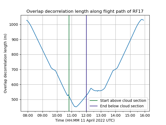
Fig. 7 Overlap decorrelation length along the flight track of RF17. The minimum can be seen at the most northerly point while the maximum is located at the end and beginning of the flight in Kiruna.

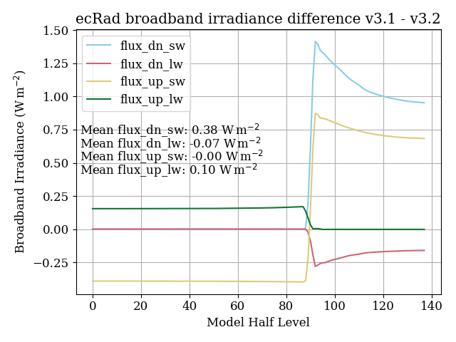
Fig. 8 ecRad broadband irradiance difference between v3.1 and v3.2 over model half levels.

Looking at the differences between the two simulations we can see differences in the solar downward flux of over \(1.25\,\text{W}\,\text{m}^{-2}\). The values used to calculate the difference are the means of the 33 columns simulated. However, the plot would not look any different even when only one column is selected.

The difference starts to increase with the simulated cloud top showing the influence of the cloud overlap decorrelation length even for single layer clouds. Thus, it is important to choose a realistic value for the case study when HALO flew first above and then below the cirrus. One option is to calculate the cloud overlap parameter \(\alpha\) according to Eq. 2.3 of the ecRad documentation:

\[\alpha_{i+\frac{1}{2}} = \frac{C_{\text{rand}} - C}{C_{\text{max}} -C}\]

with \(i\) being the model level, \(C\) being the true combined cloud cover of \(i\) and \(i+1\) and \(C_{\text{rand}}\) and \(C_{\text{max}}\) the combined cloud covers assuming random and maximum overlap respectively. See Eq. 2.4 and Eq. 2.5 of the ecRad Documentation for details. This would make the parameterization of the cloud overlap via the cloud overlap decorrelation length obsolete and cloud overlap could be provided for each timestep with the input netCDF file. However, \(C\) cannot be known from model data alone and thus the overlap parameter cannot be calculated.

The other option is to use the mean cloud overlap decorrelation length calculated for the case study period.

Case study period for RF17: 2022-04-11 10:48:47 - 2022-04-11 12:00:32

Mean cloud overlap decorrelation length for case study period: 482.87 m

Case study period for RF18: 2022-04-12 11:03:36 - 2022-04-12 12:15:45

Mean overlap decorrelation length for case study period: 453.10 m

author: Johannes Röttenbacher

Varcloud retrieval input experiment

Script: experiments.ecrad_write_input_files_v2.py

author: Johannes Röttenbacher

created: 23-03-2023

Use a processed IFS output file and the Varcloud retrieval from Florian Ewald, LMU and generate one ecRad input file for each time step along the flight path of HALO. Instead of the CIWC and \(r_{eff, ice}\) from the IFS use the retrieved variables from the Varcloud lidar/radar retrieval.

Required User Input:

All options can be set in the script or given as command line key=value pairs. The first possible option is the default.

• campaign (halo-ac3, cirrus-hl)

• key (RF17), flight key

• t_interp (False), interpolate time or use the closest time step

• init_time (00, 12, yesterday), initialization time of the IFS model run

Output:

• well documented ecRad input file in netCDF format for each time step with retrieved CIWC and \(re_{eff, ice}\)

Script: experiments.ecrad_experiment_v8.py

author: Johannes Röttenbacher

created: 24-03-2023

Comparison between using the VarCloud retrieval for IWC and \(r_{eff, ice}\) or the forecasted values from the IFS as input for an ecRad simulation using the Fu-IFS ice optic parameterization.

• IFS_namelist_jr_20220411_v1.nam: for flight HALO-AC3_20220411_HALO_RF17 with Fu-IFS ice model

• IFS_namelist_jr_20220411_v8.nam: for flight HALO-AC3_20220411_HALO_RF17 with Fu-IFS ice model and VarCloud input

Focus is on the above cloud section in the high north before the below cloud section where no VarCloud retrieval is available anymore.

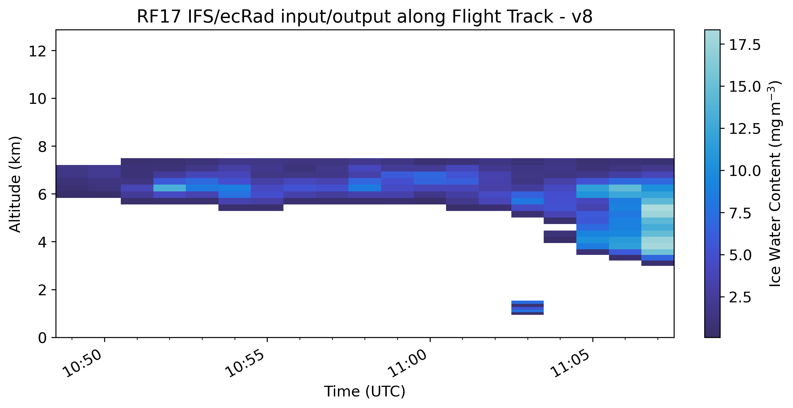
Fig. 9 Retrieved ice water content from VarCloud retrieval interpolated to IFS full level pressure altitudes.

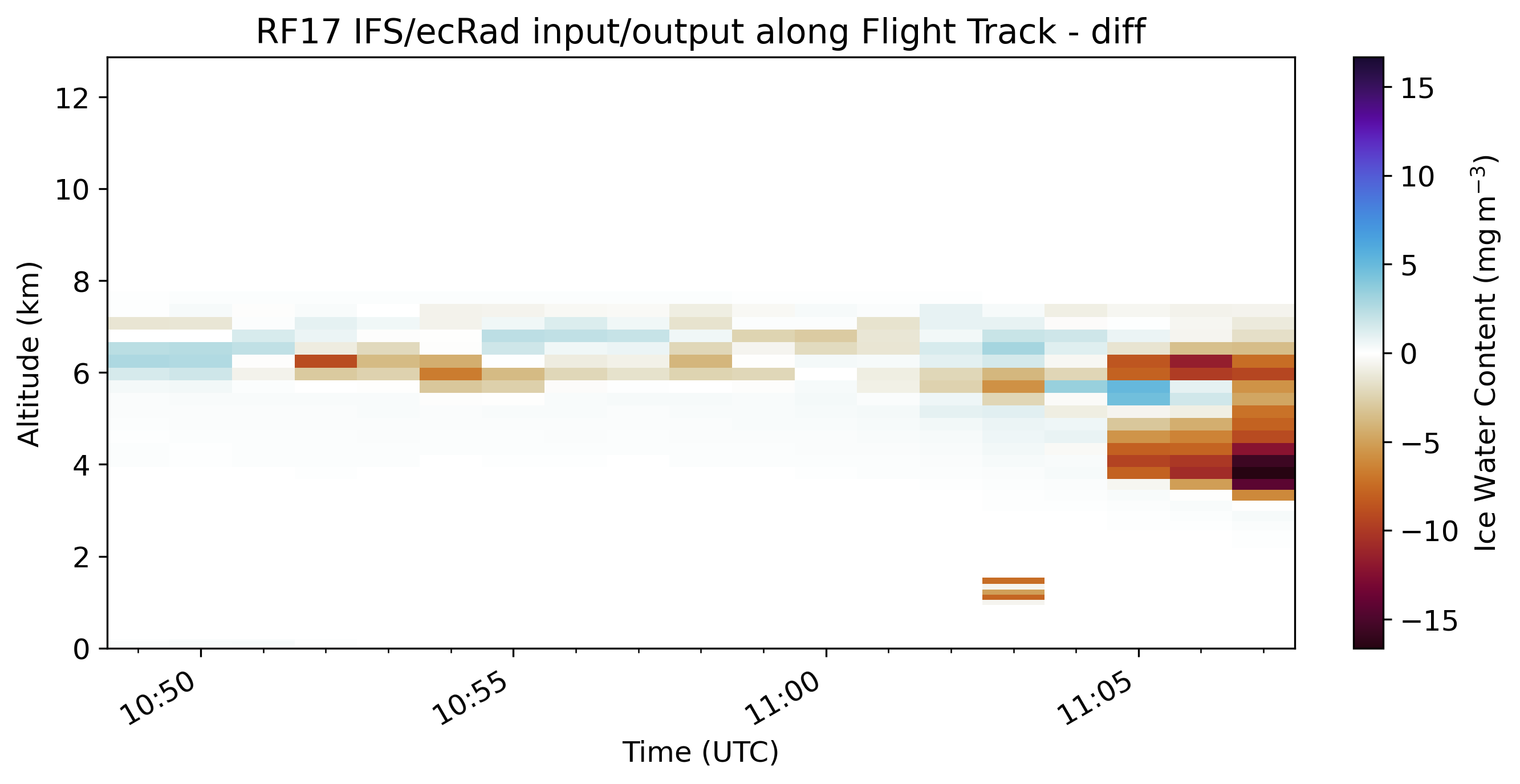
Fig. 10 Difference between IWC IFS and IWC VarCloud.

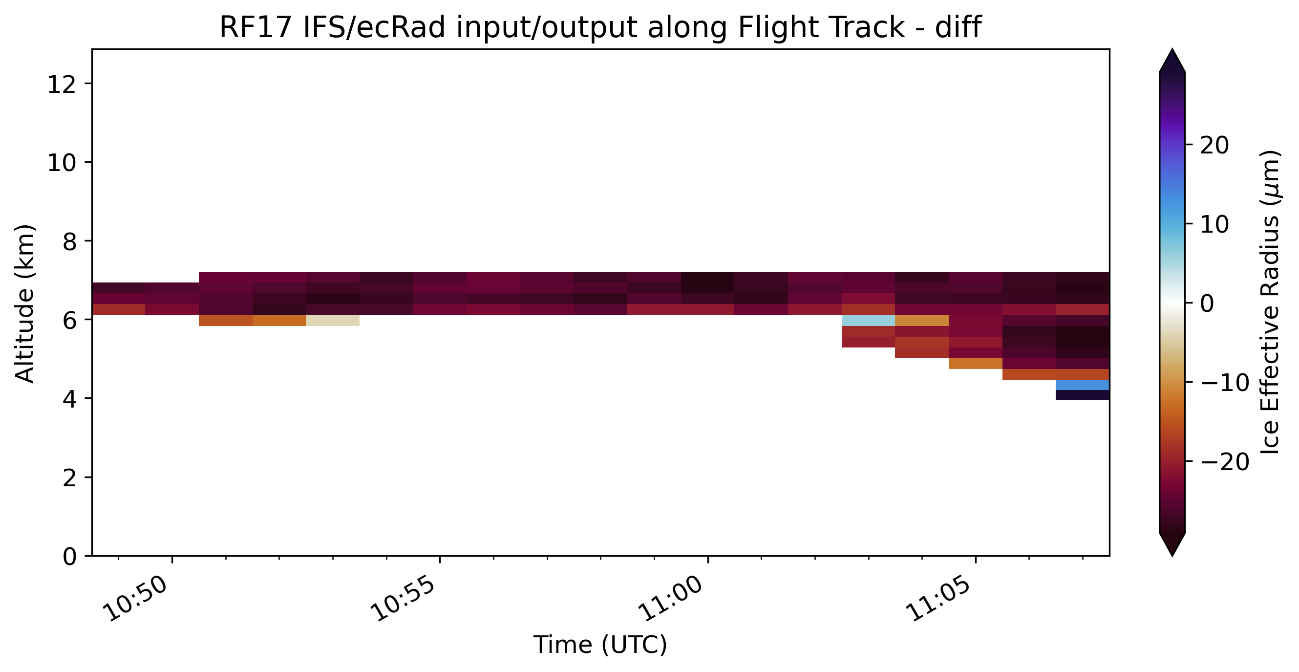
Fig. 11 Difference between \(r_{eff, ice}\) IFS and \(r_{eff, ice}\) VarCloud.

From the two figures above it can be seen that the VarCloud retrieval produces a higher IWC and larger \(r_{eff, ice}\). The histograms show the same picture.

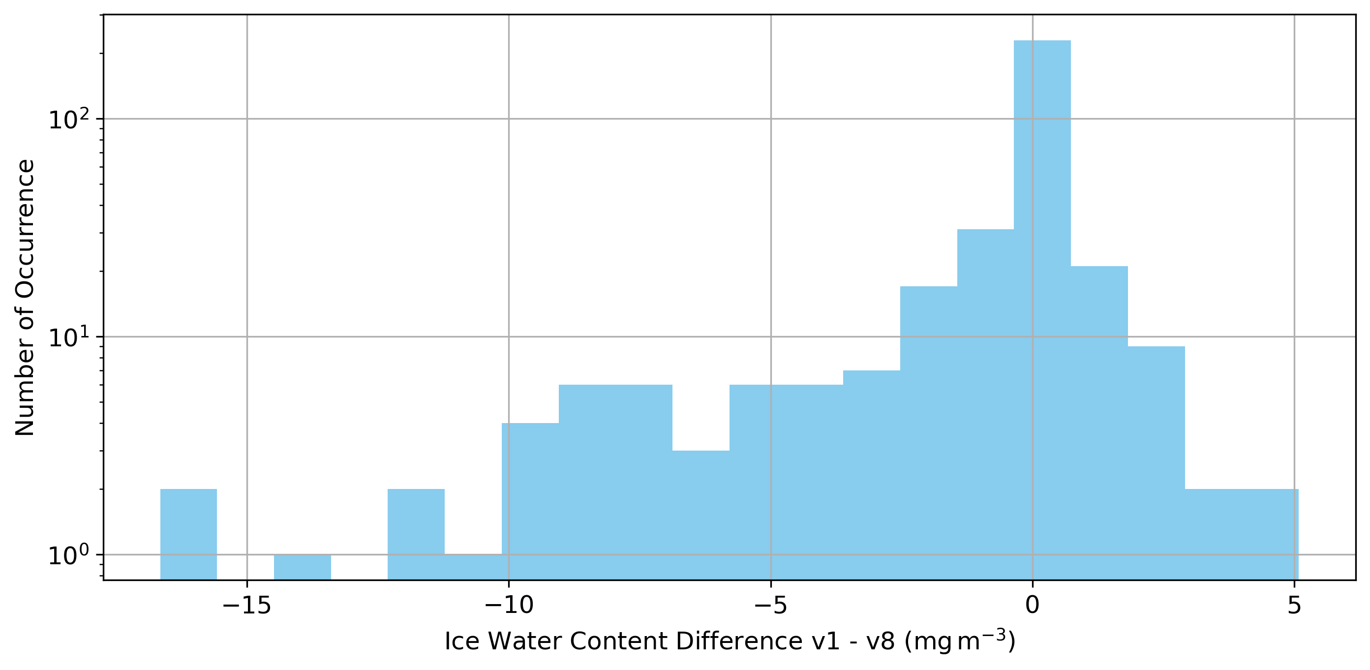
Fig. 12 Histogramm of difference between IWC IFS and IWC VarCloud.

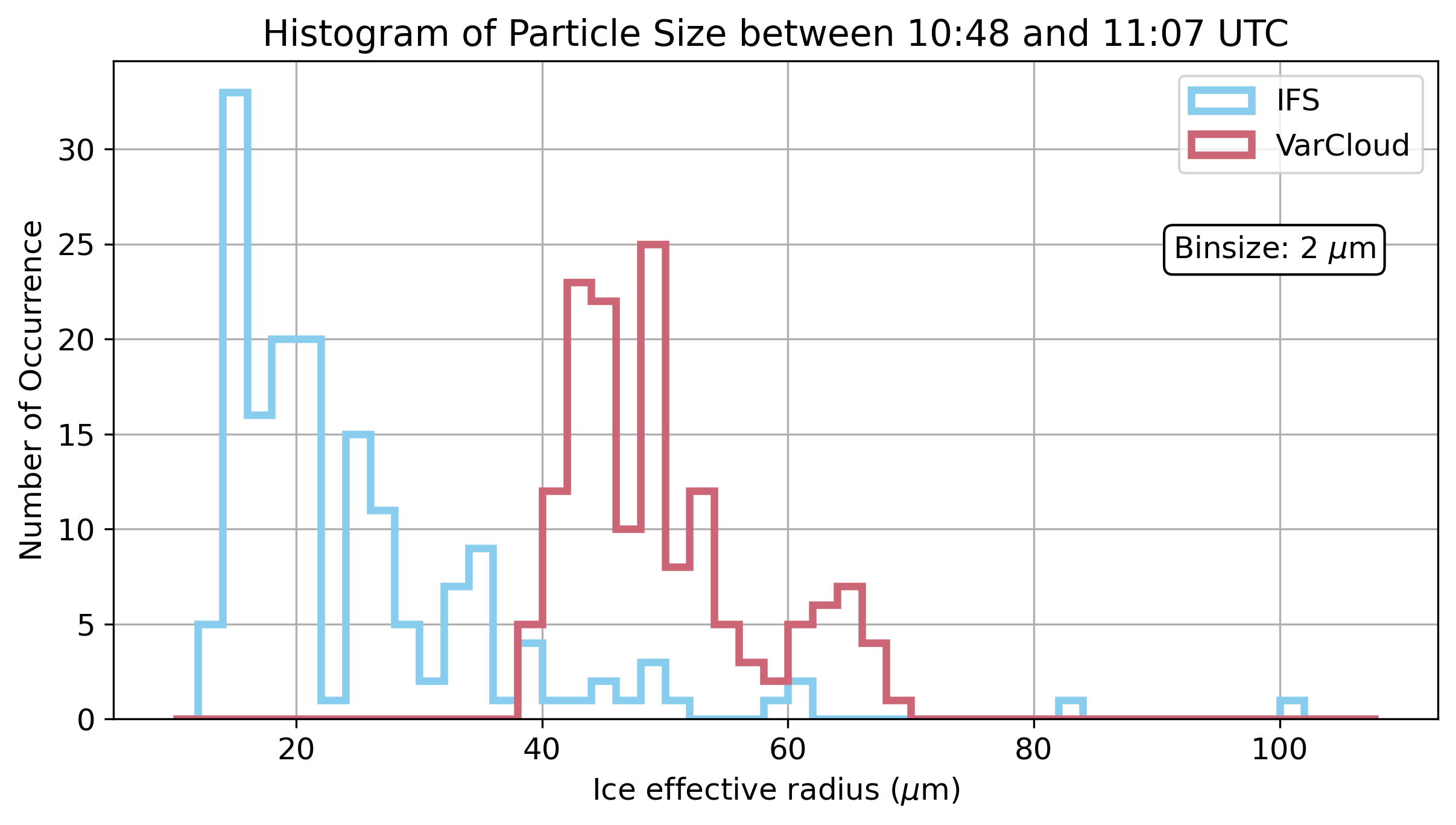
Fig. 13 Histogramm of \(r_{eff, ice}\) used in the IFS run and the VarCloud run.

The differences in microphysical properties also translate to differences in optical properties of the cloud such as higher total optical depth (integrated over all bands) in the IFS run.

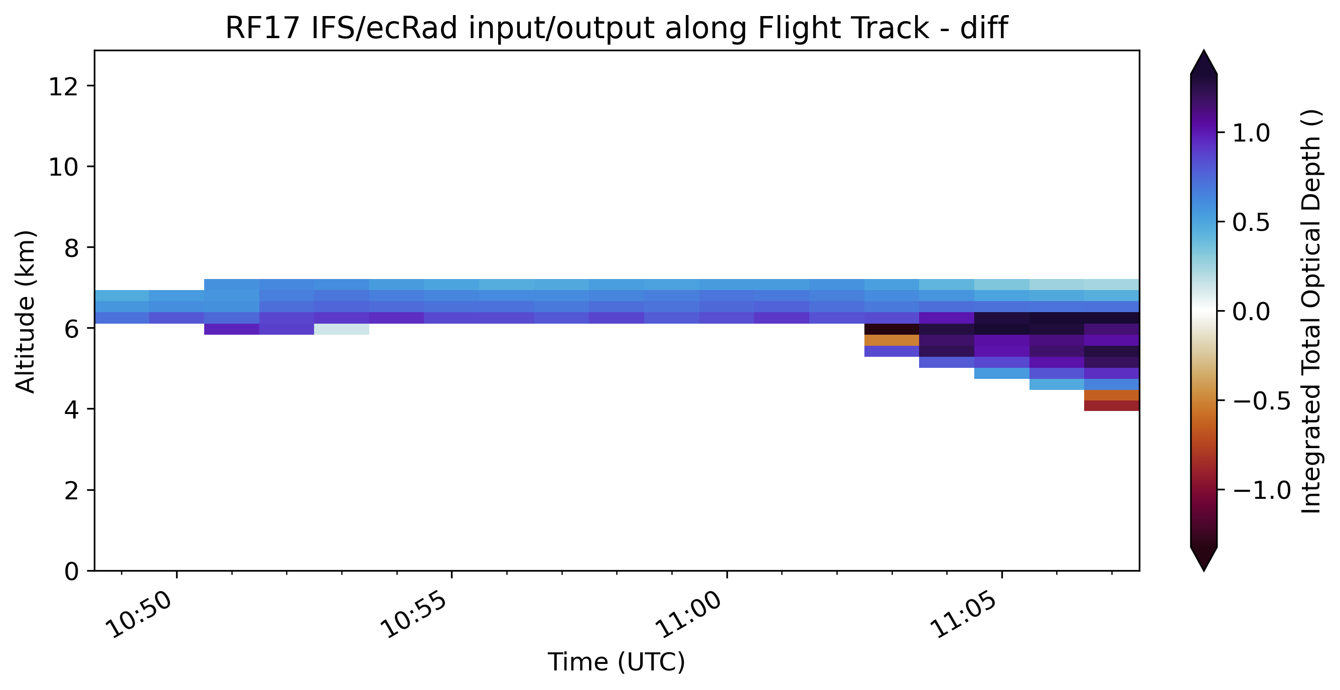
Fig. 14 Difference in total optical depth integrated over all shortwave bands between the IFS run and the VarCloud run.

Finally, due to larger \(r_{eff, ice}\) the ice cloud from the retrieval is less absorbing/reflecting than the IFS forecasted ice cloud.

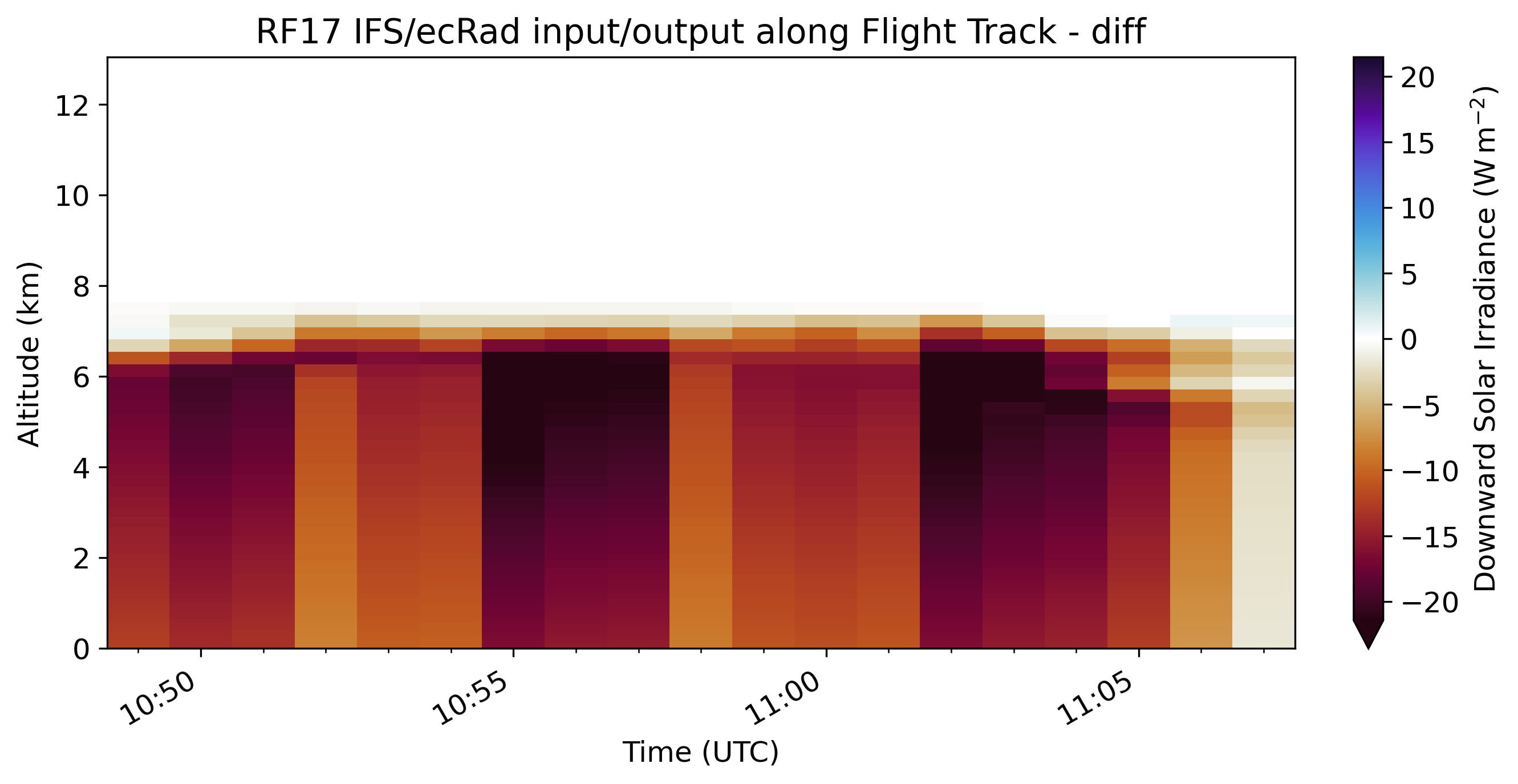
Fig. 15 Difference in broadband solar downward irradiance between IFS and VarCloud.

Fig. 16 Histogramm of difference in broadband solar downward irradiance between IFS and VarCloud.

Ice Mass Mixing Ratio Experiment

Script: experiments.ecrad_write_input_files_v4.py

author: Johannes Röttenbacher

created: 05-04-2023

Instead of summing up Cloud Ice Water Content (ciwc) and Cloud Snow Water Content (cswc) for the ice mass mixing ratio (\(q_{ice}\)), use only ciwc as \(q_{ice}\).

Required User Input:

All options can be set in the script or given as command line key=value pairs. The first possible option is the default.

• key (RF17), flight key

• t_interp (False), interpolate time or use the closest time step

• init_time (00, 12, yesterday), initialization time of the IFS model run

Output:

• well documented ecRad input file in netCDF format for each time step with q_ice = ciwc

Script: experiments.ecrad_experiment_v11.py

author: Johannes Röttenbacher

created: 05-04-2023

Analyze the impact of using only Cloud Ice Water Content (ciwc) as ice mass mixing ratio (\(q_{ice}\)) instead of summing up ciwc and Cloud Snow Water Content (cswc) for \(q_{ice}\).

• IFS_namelist_jr_20220411_v1.nam: for flight RF17 with Fu-IFS ice model

• IFS_namelist_jr_20220411_v11.nam: for flight RF17 with Fu-IFS ice model and ciwc as q_ice

Problem statement: Using the Varcloud retrieval as input for IWC (converted to \(q_{ice}\)) seemed to explain the overestimation of optical depth in the IFS. However, RF18 did not show the same bias in downward solar irradiance below the cloud as RF17. One possible reason to explain this inconsistency could be the cswc which increased the clouds size in both cases but more so in RF18. Thus, we investigate the impact of removing it from the simulation.

Focus is on the case study in the high north. First let’s look at the difference in \(q_{ice}\) for v1 where \(q_{ice} = ciwc + cswc\) and v11 where \(q_{ice} = ciwc\).

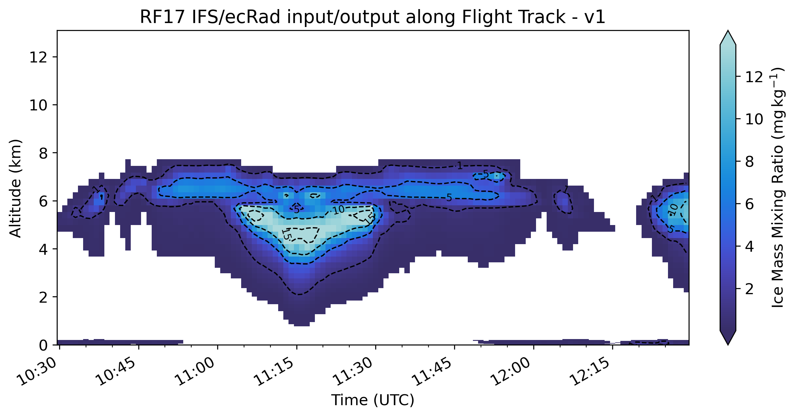
Fig. 17 Ice mass mixing ration for v1.

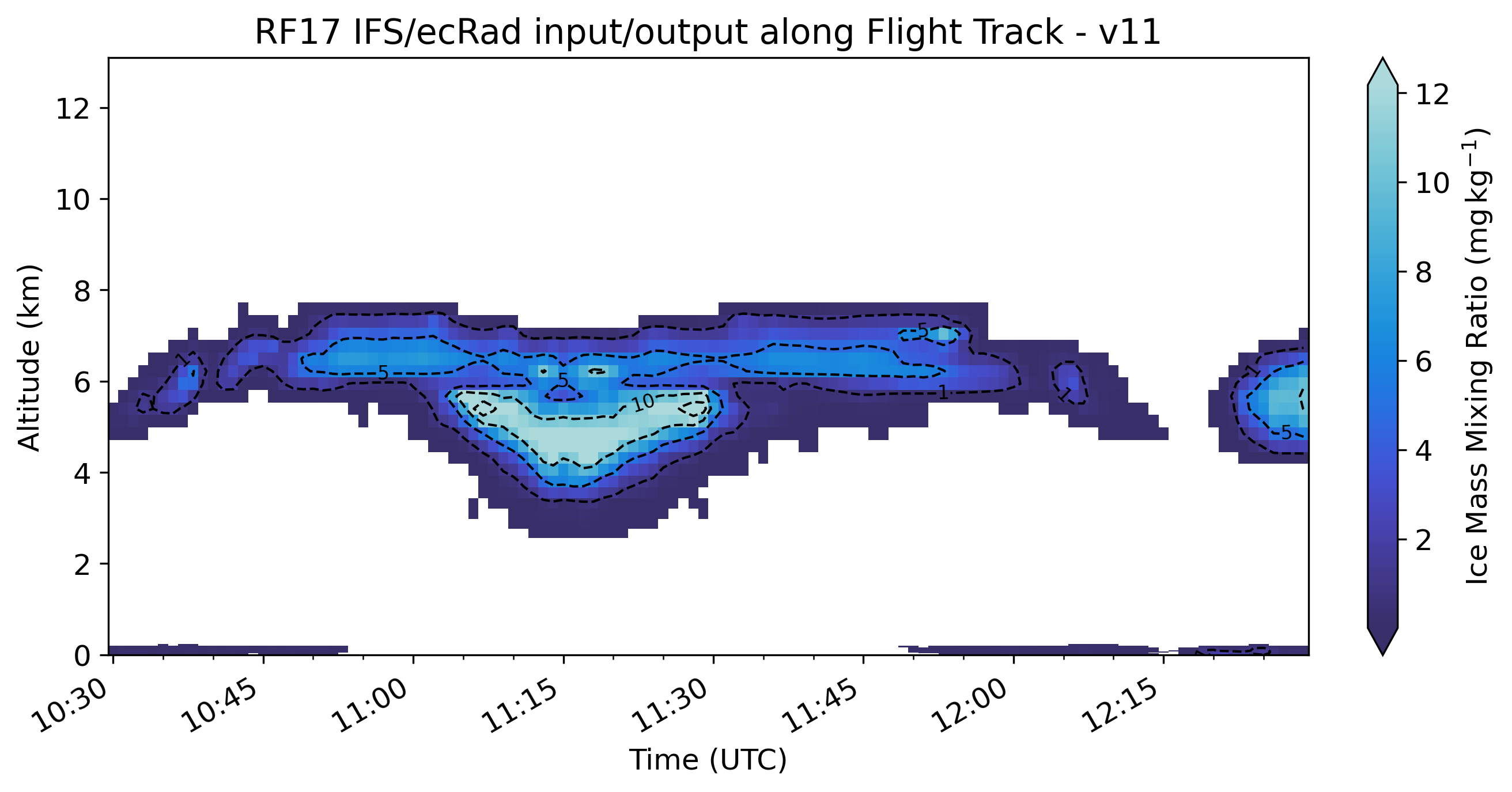
Fig. 18 Ice mass mixing ration for v11.

The interesting question is now if ecRad also sees a cloud with the extent of \(q_{ice}\) in v1. It could well be that it doesn’t because there is no \(r_{eff, ice}\) simulated there. Or to be more precise only a fill value (5.196162e-05) is set.

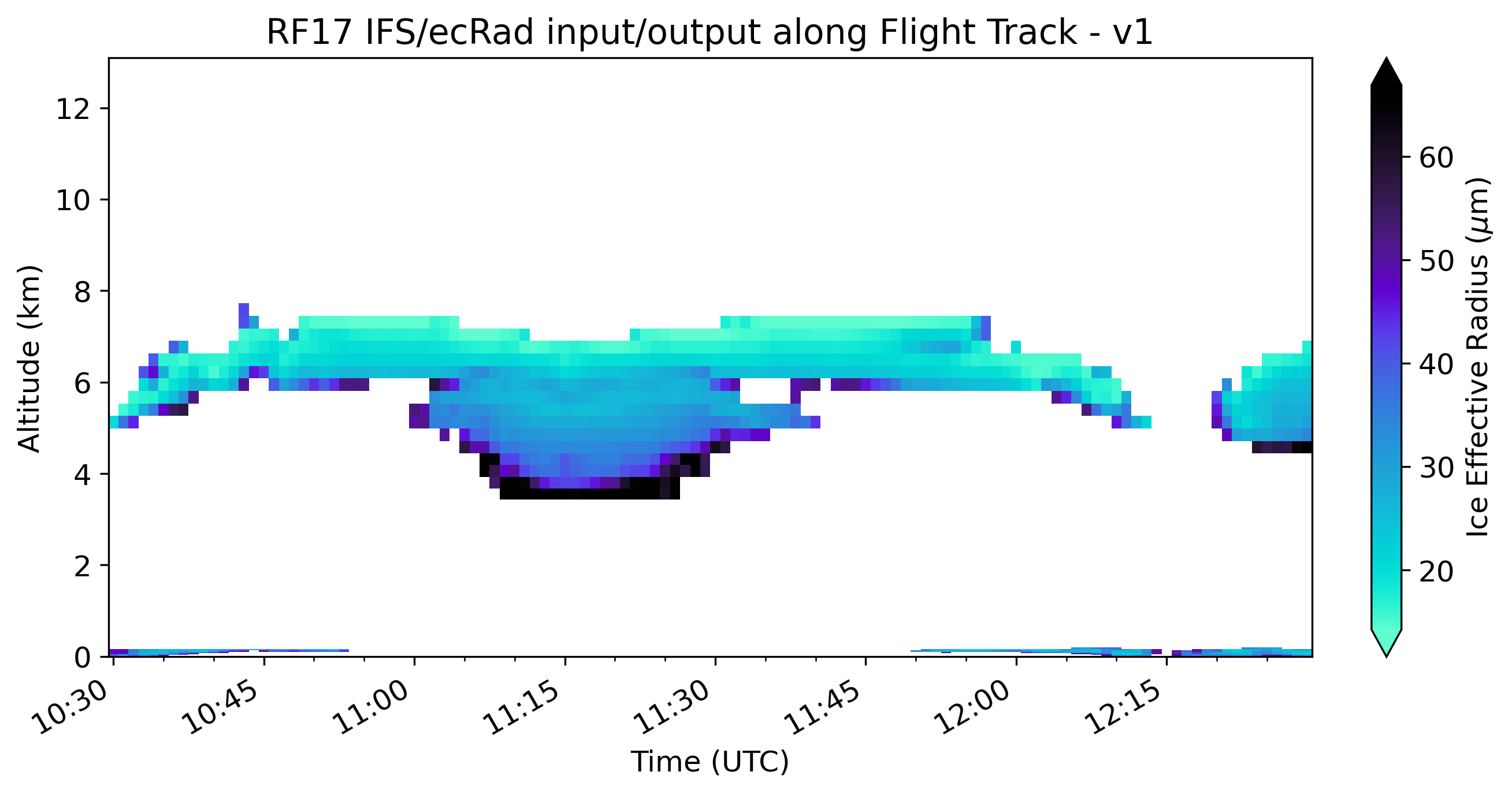
Fig. 19 Ice effective radius for v1. White areas are filled with a fill value for the simulation.

Let’s take a look at the difference in downward solar irradiance for the case study period (v1 - v11).

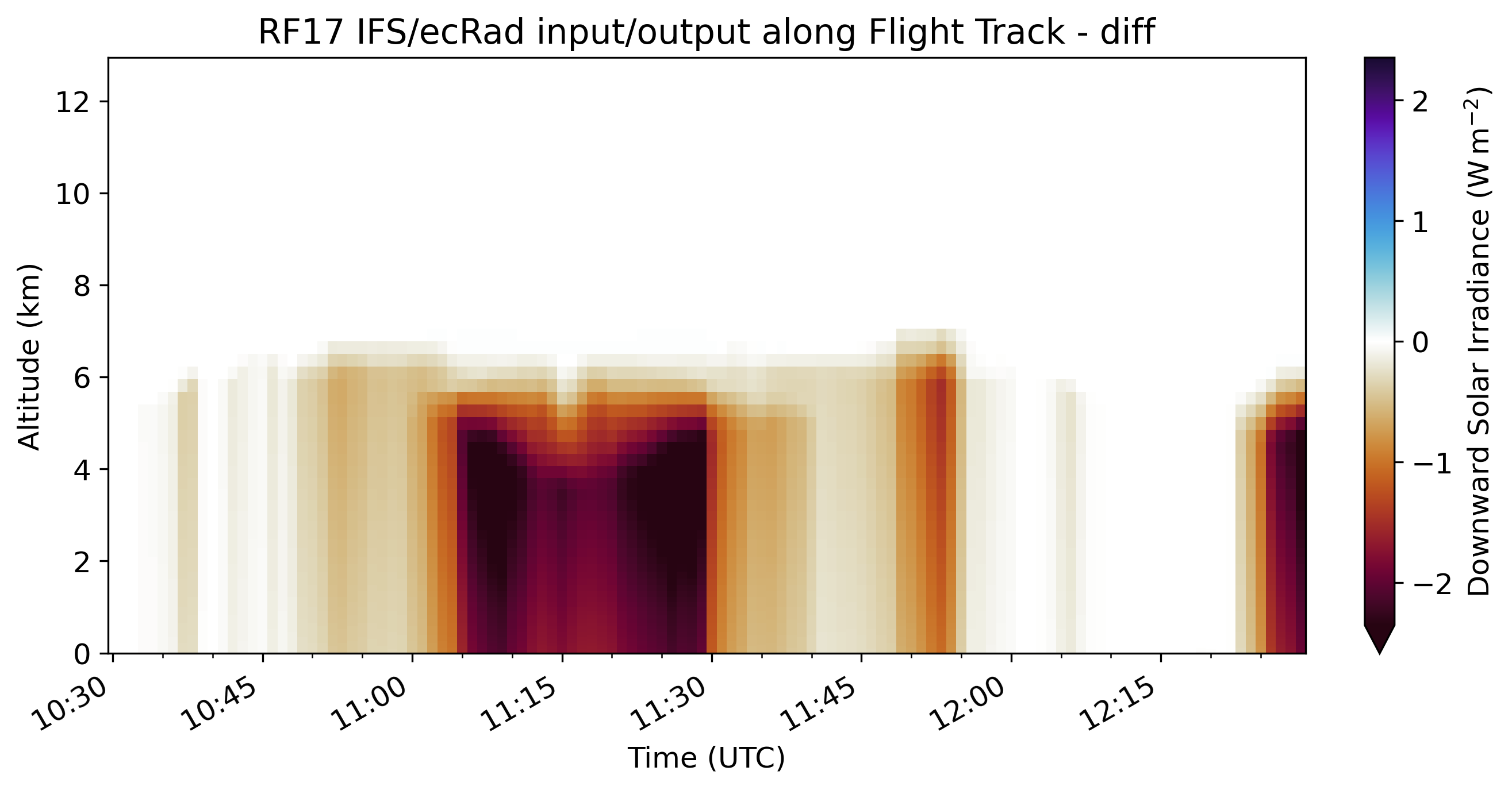
Fig. 20 Difference in downward solar irradiance between v1 and v11.

The difference here seems to come from the \(q_{ice}\) difference in the core of the cloud (see Fig. 21).

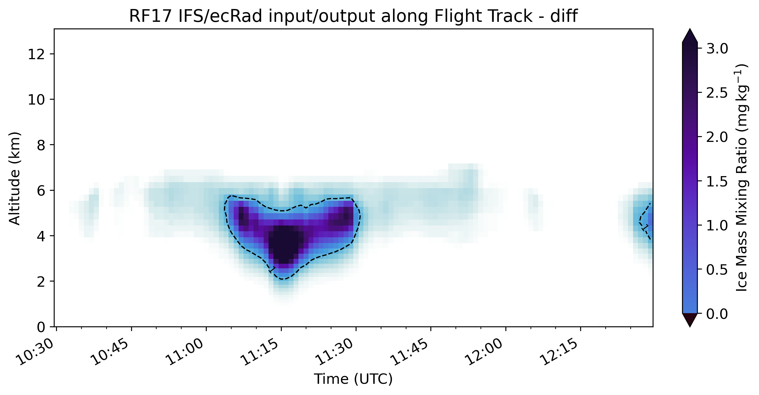
Fig. 21 Difference in \(q_{ice}\) between v1 and v11.

So although the cswc increases the size of the cloud it does not affect the simulation outside the cloud since there is no \(r_{eff, ice}\) simulated there. It, thus, only increases \(q_{ice}\) inside the actual cloud which leads to higher optical depth of the cloud and thus more scattering/absorption. This can be seen in the reduced downward solar irradiance below the cloud in Fig. 20.

Fixed Albedo Experiment

Input files for ecRad

Script: experiments.ecrad_write_input_files_v5.py

author: Johannes Röttenbacher

created: 15-04-2023

Replace sw_albedo calculated according to Ebert and Curry [1993] with open ocean albedo (0.06) for the whole flight.

Required User Input:

All options can be set in the script or given as command line key=value pairs. The first possible option is the default.

• key (RF17), flight key

• t_interp (False), interpolate time or use the closest time step

• init_time (00, 12, yesterday), initialization time of the IFS model run

Output:

• well documented ecRad input file in netCDF format for each time step with sw_albedo = 0.06

Script: experiments.ecrad_write_input_files_v5_1.py

author: Johannes Röttenbacher

created: 15-04-2023

Replace sw_albedo calculated according to Ebert and Curry [1993] with a maximum albedo (0.99) for the whole flight and scale all bands according to the differences in the original sw_albedo.

Required User Input:

All options can be set in the script or given as command line key=value pairs. The first possible option is the default.

• key (RF17), flight key

• t_interp (False), interpolate time or use the closest time step

• init_time (00, 12, yesterday), initialization time of the IFS model run

Output:

• well documented ecRad input file in netCDF format for each time step with scaled sw_albedo and a maximum of 0.99

Script: experiments.ecrad_write_input_files_v5_2.py

author: Johannes Röttenbacher

created: 05-09-2023

Scale the BACARDI measured broadband albedo for the below cloud section with the sw_albedo calculated according to Ebert and Curry [1993].

Required User Input:

All options can be set in the script or given as command line key=value pairs. The first possible option is the default.

• key (RF17), flight key

• t_interp (False), interpolate time or use the closest time step

• init_time (00, 12, yesterday), initialization time of the IFS model run

Output:

• well documented ecRad input file in netCDF format for each time step below cloud with sw_albedo according to the BACARDI measurement

Analysis

Script: experiments.ecrad_experiment_v13.py

author: Johannes Röttenbacher

created: 15-04-2023

Set the albedo during the whole flight to open ocean (diffuse: 0.06, direct: Taylor et al. 1996) or scale it to 0.99 (maximum albedo) and analyze the impact on the offset between simulation and measurement during the below cloud section of RF17.

• IFS_namelist_jr_20220411_v13.nam: for flight RF17 with Fu-IFS ice model setting albedo to open ocean (input version v5)

• IFS_namelist_jr_20220411_v13.1.nam: for flight RF17 with Fu-IFS ice model setting albedo to 0.99 (input version v5.1)

• IFS_namelist_jr_20220411_v13.2.nam: for flight RF17 with Fu-IFS ice model setting albedo BACARDI measurement from below cloud section (input version v5.2)

• IFS_namelist_jr_20220411_v15.1.nam:: for RF17 with Fu-IFS ice model using O1280 IFS data (input version v6.1) (reference simulation)

Problem statement: A clear offset can be observed in the solar downward irradiance below the cloud between ecRad and BACARDI with ecRad showing lower values than BACARDI. One idea is that multiple scattering from the sea ice surface to the cloud and back down plays is a process not captured by the model. By setting the albedo to open ocean we can eliminate this multiple backscattering between cloud and surface. Comparing this experiment with the standard experiment can show us the potential impact of multiple scattering. We also run an experiment where we scale the albedo to 0.99 to see how much more downward irradiance we can observe that way.

Extension: We extend the analysis and use the scaled measured below cloud albedo from BACARDI as input.

We will focus on the above and below cloud section in the far north. The corresponding spectral surface albedo as used in the IFS can be seen in Fig. 22.

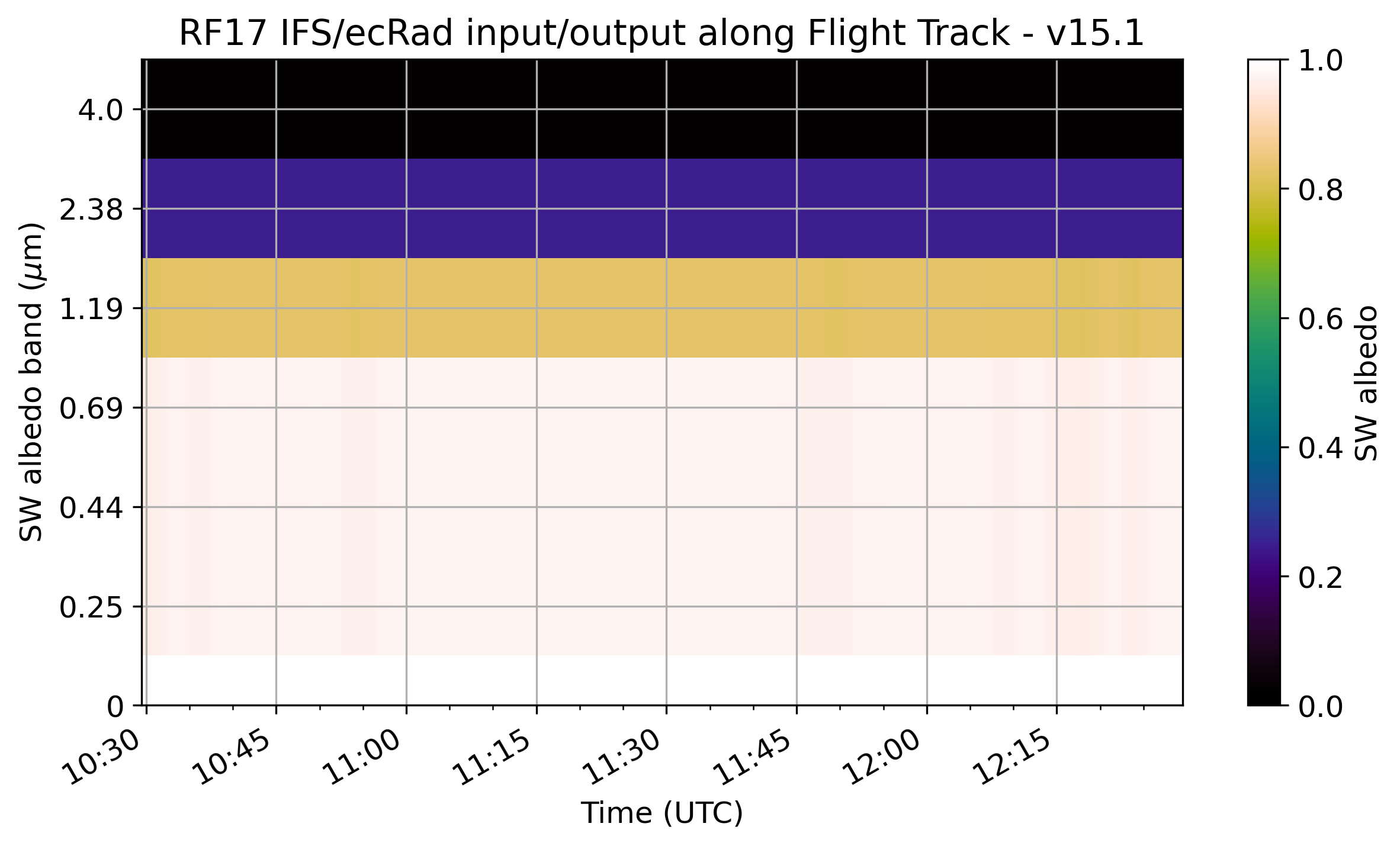
Fig. 22 Short wave albedo along track above and below cloud for all six spectral bands after Ebert and Curry [1993].

At first, we look at the difference in solar upward and downward irradiance between v15.1 (IFS albedo after Ebert and Curry [1993]) and v13 (ocean albedo).

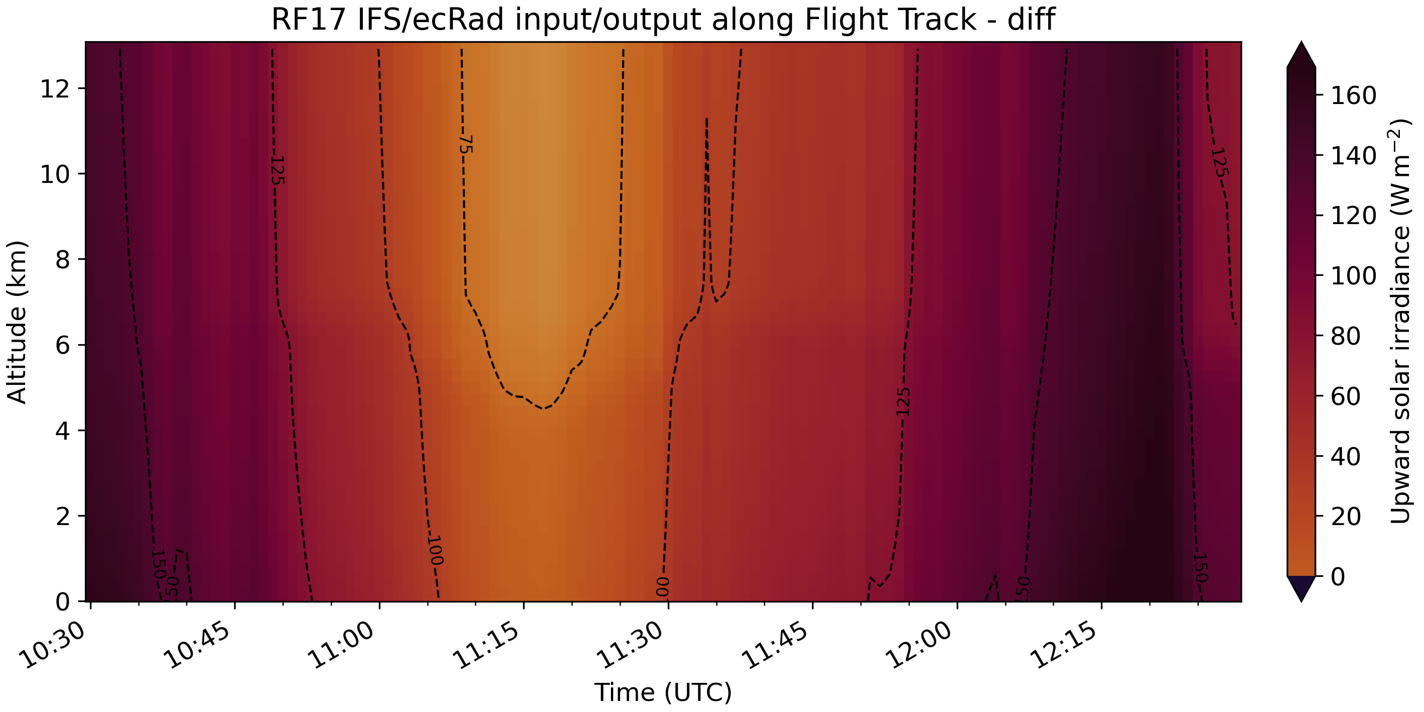
Fig. 23 Difference in solar upward irradiance between v15.1 and v13.

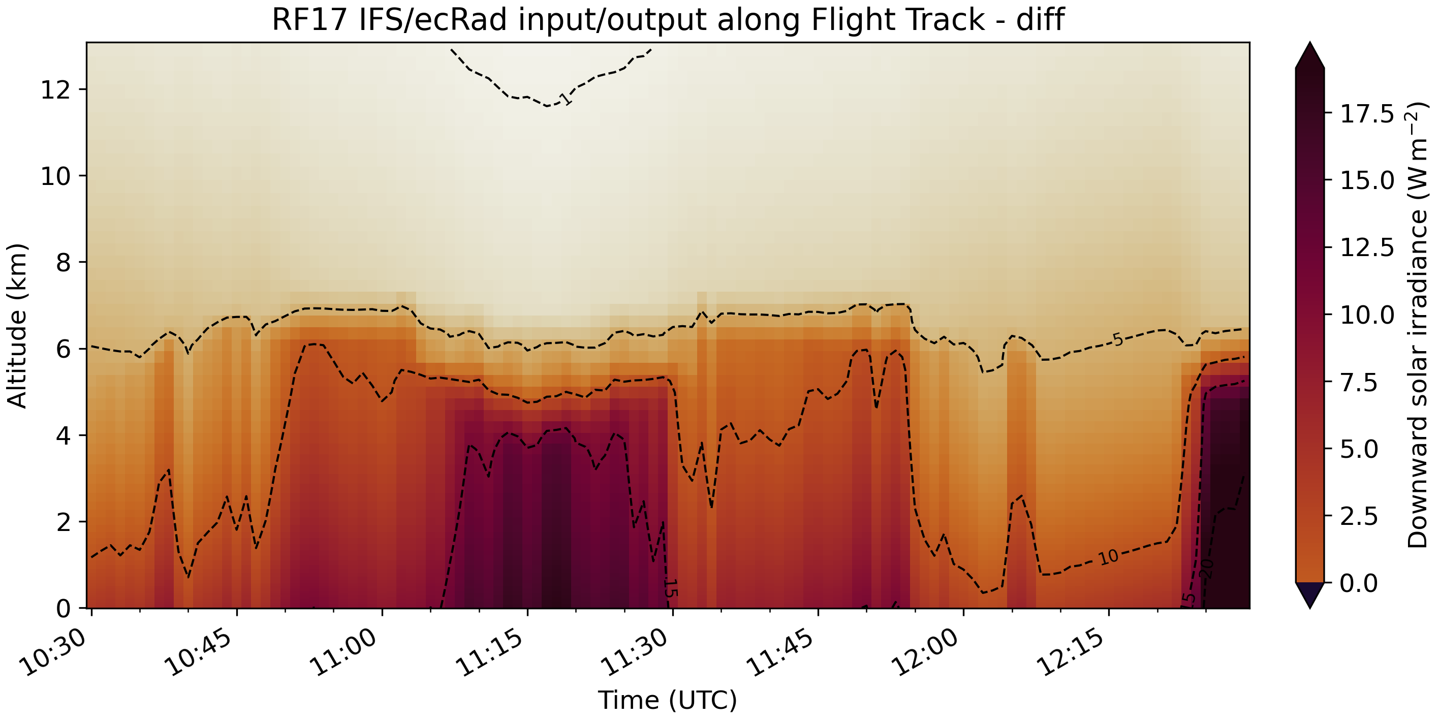
Fig. 24 Difference in solar downward irradiance between v15.1 and v13.

We can see an unsurprising substantial difference in upward irradiance which then propagates to a smaller but still relevant difference in downward irradiance. This is especially pronounced for the thicker section of the cirrus at around 11:15 UTC.

An interesting side note: Although the surface albedo is now set to an open ocean value the emissivity and skin temperature are still the same. Thus, there is only a minor change in the terrestrial upward irradiance.

So how much difference does multiple scattering between the surface and cloud make? For this we can take a look at the histogramm of differences and some statistics.

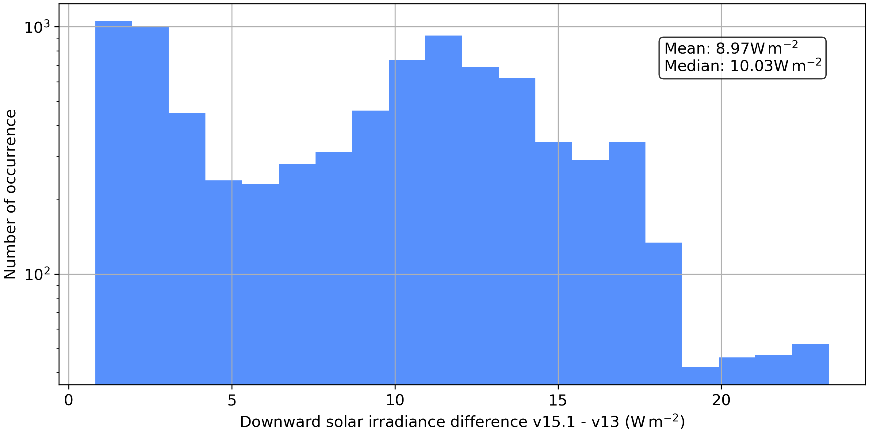
Fig. 25 Histogram of differences between v15.1 and v13.

We see that a lot of values are rather small. They correspond to the area above the cloud where only the atmosphere causes some minor scattering. The median and mean of the distribution, however, are around \(10\,Wm^{-2}\), which is quite substantial.

So albedo does obviously have a major influence on the downward irradiance in this scenario. The next question now is, whether we can reduce the bias by increasing the surface albedo? For this we take a look at experiment v13.1 with a scaled albedo of 0.99. The albedo is scaled in such a way that the maximum albedo in the first short wave albedo band is set to 0.99 and the following bands are scaled according to the relative differences between the original short wave albedo bands. See the script for details.

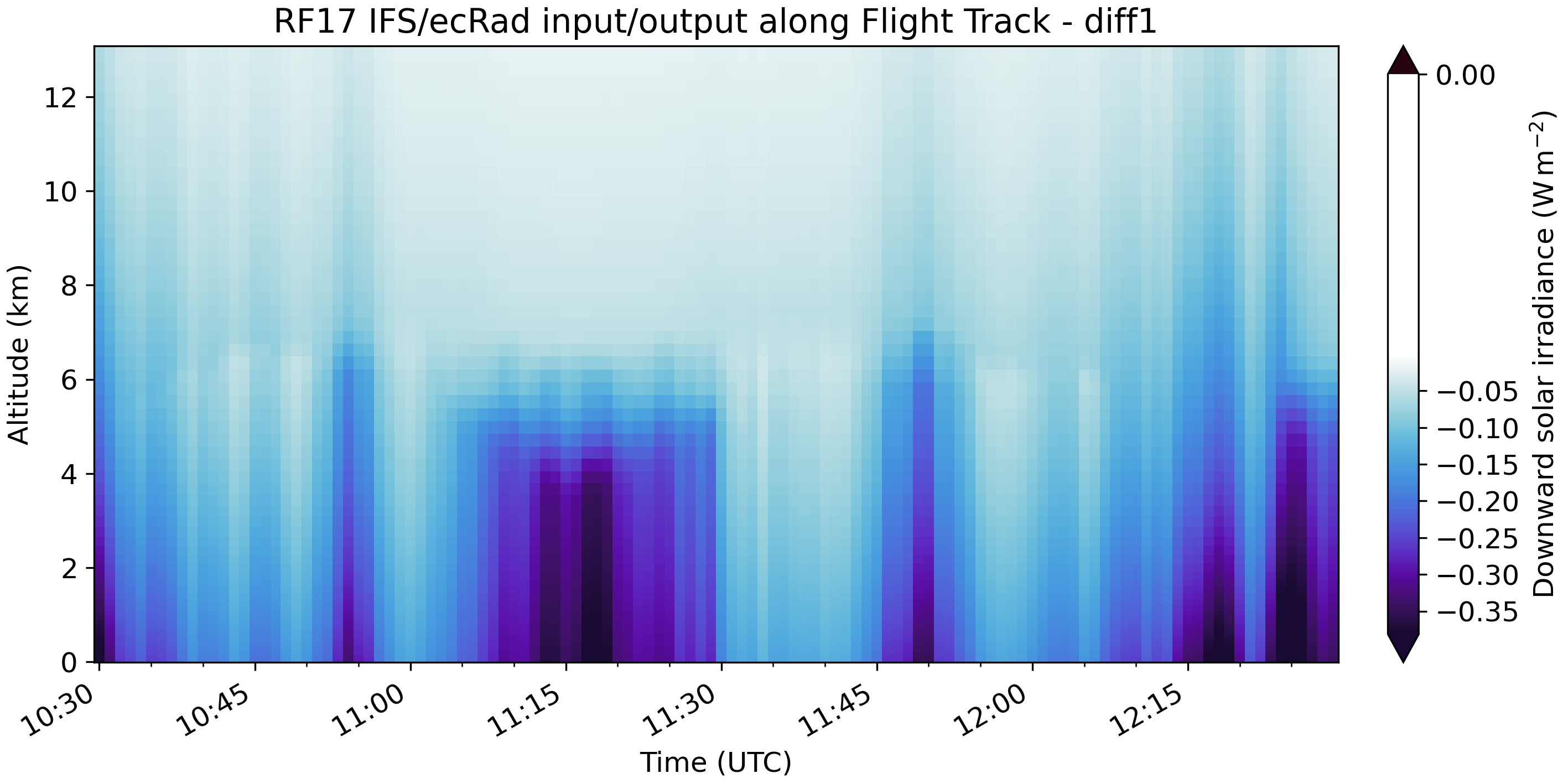
Fig. 26 Difference in solar downward irradiance between v15.1 and v13.1 (albedo = 0.99).

By scaling the albedo to an unrealistic value of 0.99 we get a maximum of \(0.45\,Wm^{-2}\) difference in solar downward irradiance. Comparing the spectral albedo of each experiment in Fig. 27 we can also see, that the standard albedo for the scene is already high. So increasing it does not seem to be a sensible idea.

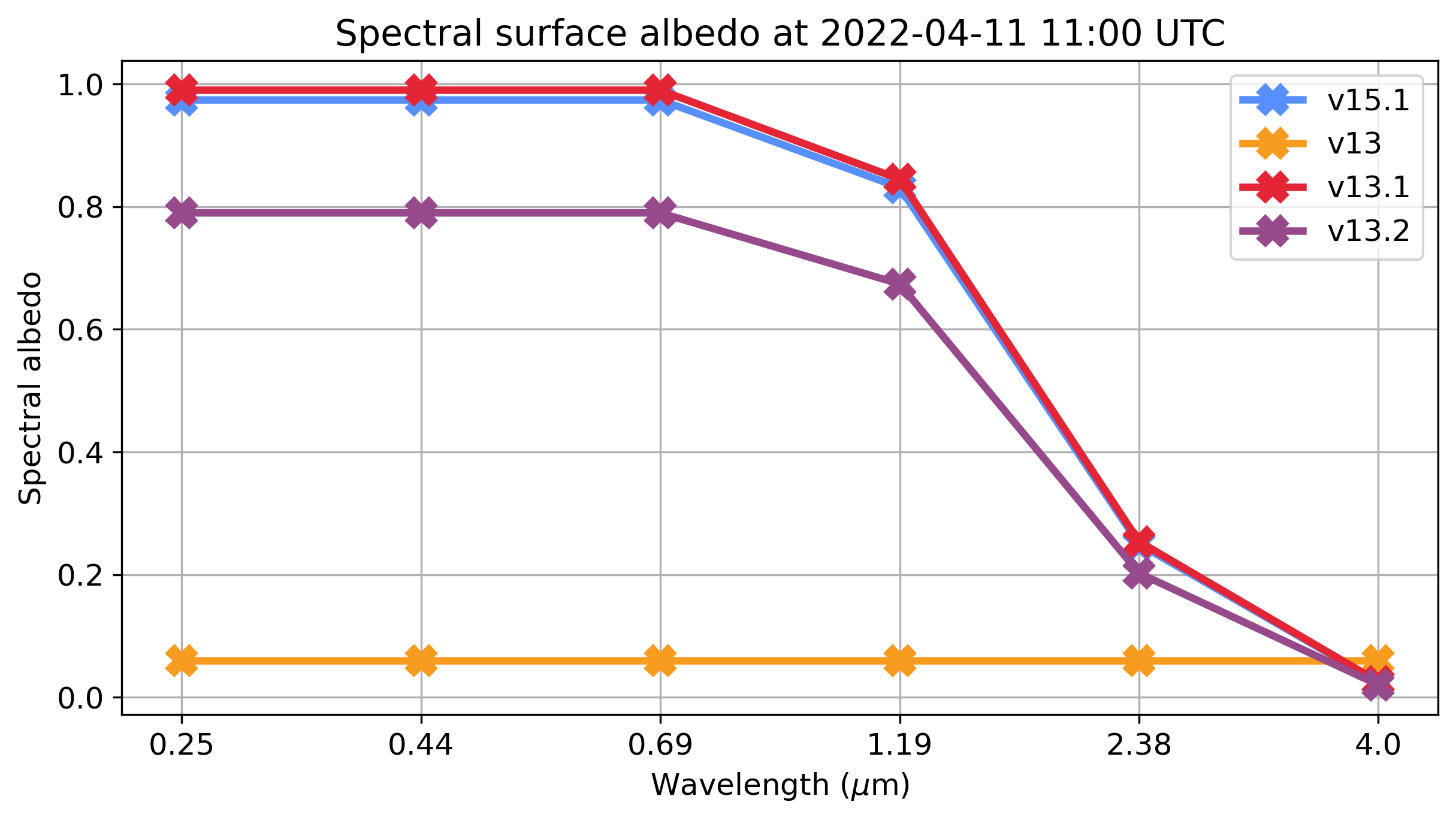
Fig. 27 Spectral albedo for all four experiments at one timestep below cloud.

However, what happens if we use the measured broadband albedo from BACARDI for the below cloud simulation which is lower than the one in the IFS but not as low as for open ocean?

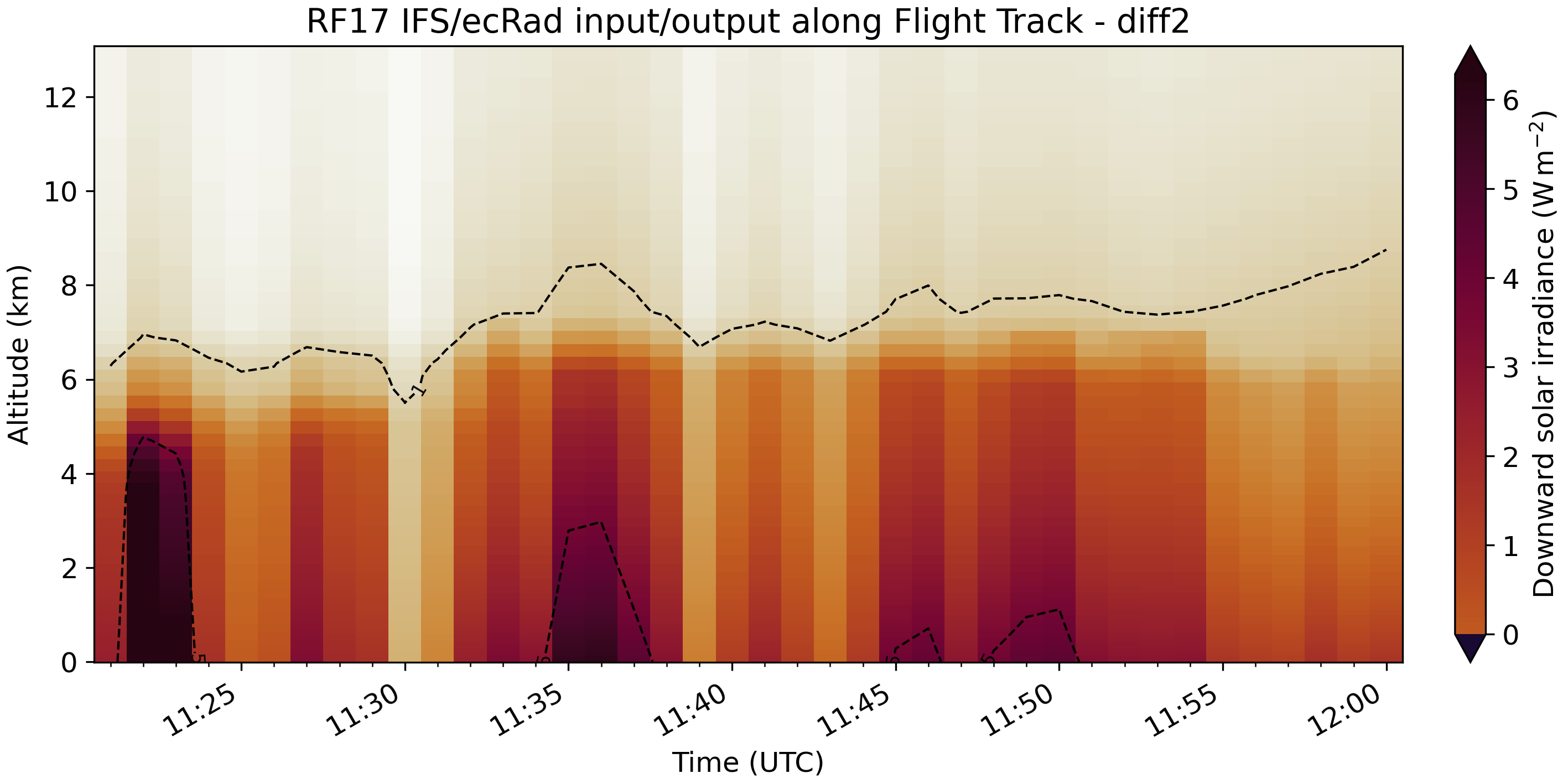
Fig. 28 Difference in solar downward irradiance between v15.1 and v13.2 (albedo from BACARDI).

Looking at the difference in solar downward irradiance we can see that it is still a positive difference meaning the predicted downward irradiance is still smaller compared to the IFS run. The comparison with the measurements also shows a worse match compared to v15.1.

From all this we can conclude that the albedo does not seem to be the major problem in this scene. Or at least, we cannot tweak it in any reasonable way to improve the simulations.

Trace gas comparison

Script: experiments.ecrad_trace_gases.py

author: Johannes Röttenbacher

created: 13.10.2023

Compare standard simulation (input v6, namelist v15) before and after implementing the CAMS trace gas climatology.

Input files:

• ecrad_merged_inout_20220411_v15_old.nc -> fixed trace gases, ozone sonde

• ecrad_merged_inout_20220411_v15.nc -> CAMS climatology trace gases

First, let’s compare the mean profiles of trace gases in the case study region.

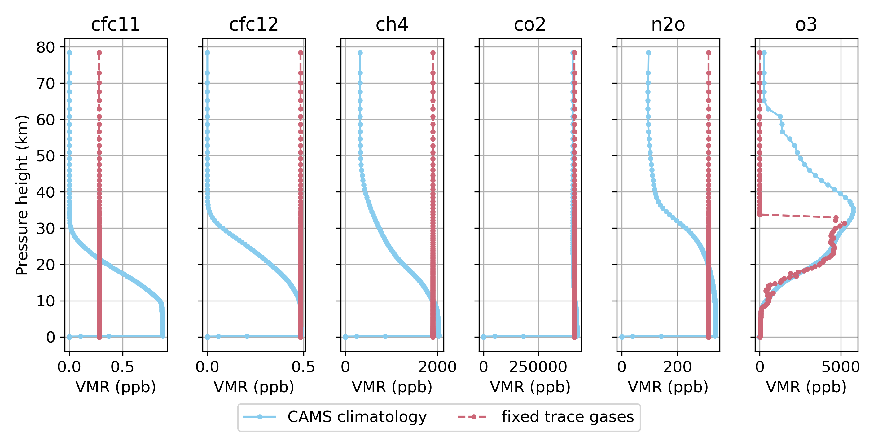
Fig. 29 Mean profiles of trace gases in the case study region. Fixed values are replicated over height.

Apart from O3 and CO2 all trace gases decrease with altitude in the CAMS climatology whereas the constant values are also high in the upper atmosphere. For CO2 there is not much difference apart from the values at ground. O3 does show a difference in the upper atomsphere where there are no more sonde measurements and the values are set to 0 in the old run. In the region where the sonde is available the climatology shows a good match. It would thus be better to use the climatology as it extends the O3 profile through the whole atmosphere. A mixture of both could also be possible.

Let’s look at the impact of the differet sources of trace gases on the radiative fluxes. We will look at the difference of new - old, so v15 - v15_old.

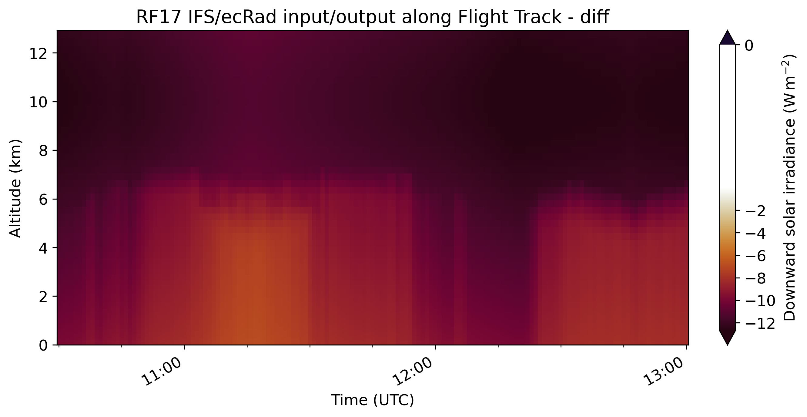
Fig. 30 Difference in solar downward irradiance between the simulations using the CAMS climatology (v15) and the ones using the fixed values (v15_old).

Especially above cloud we see a substantial difference of up to \(-12\,Wm^{-2}\).

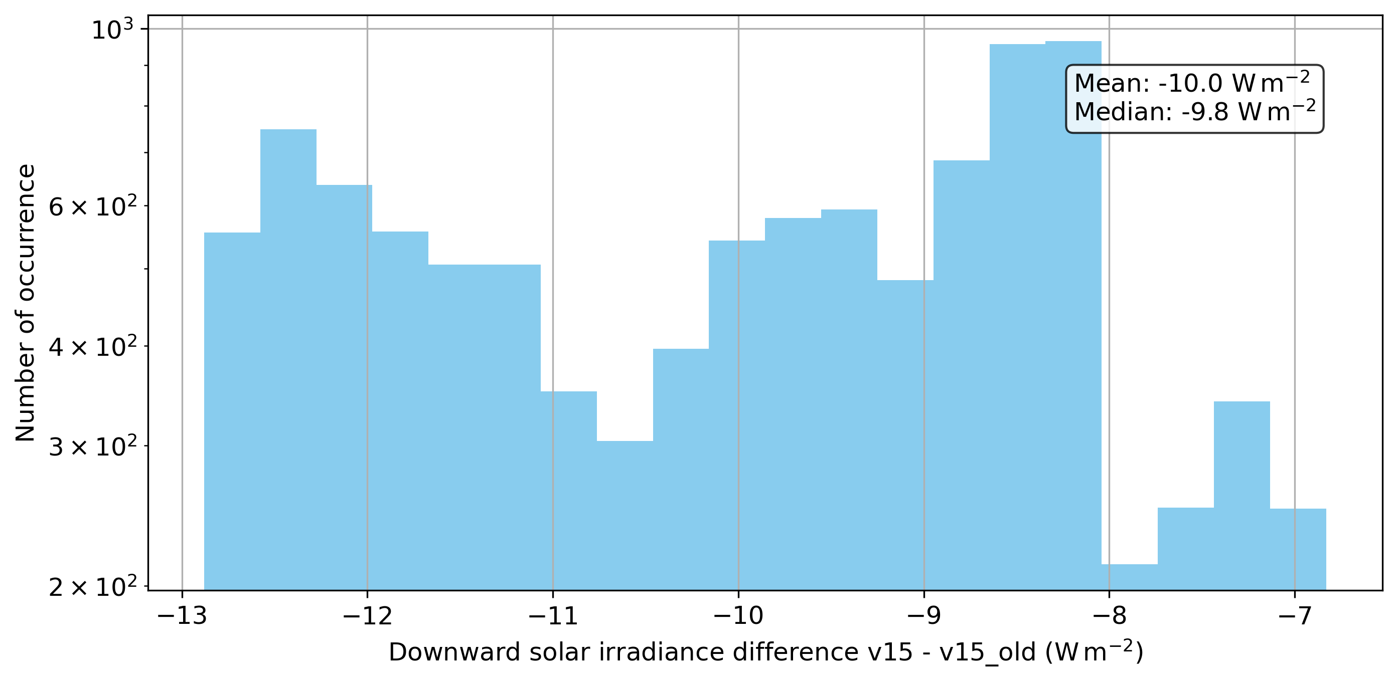
Fig. 31 Hisotgram of differences of solar downward irradiance between the simulations using the CAMS climatology (v15) and the ones using the fixed values (v15_old).

Looking at the histogram of differences we see a mean of \(-10\,Wm^{-2}\) and a minumum at \(-7\,Wm^{-2}\). From this we can conclude that more realistic profiles of trace gases in the simulations lead to less solar downward irradiance. This is probably due to more scattering in the upper atmosphere. The main cause for this is probably the ozone (O3) profile. More sensitivity studies are needed to pinpoint this, however.

Inhomogeneity test (fractional_std)

Script: experiments.ecrad_experiment_v36.py

author: Johannes Röttenbacher

created: 19-01-2024

Set the fractional standard deviation to 0. This will remove any subgrid scale variability of IWC. Thus, the cloud is homogeneous in each grid cell. Using the VarCloud input for these simulations would then have the effect of representing the measured inhomogeneity of the cloud field.

Namelists used:

• IFS_namelist_jr_20220411_v36.nam: for RF17 with Fu-IFS ice model using O1280 IFS, varcloud retrieval for ciwc and re_ice input below cloud, turned fractional standard deviation to 0 (measure for inhomogeneity) (input version v7)

• IFS_namelist_jr_20220411_v37.nam: for RF17 with Yi2013 ice model using O1280 IFS, varcloud retrieval for ciwc and re_ice input below cloud, turned fractional standard deviation to 0 (measure for inhomogeneity) (input version v7)

• IFS_namelist_jr_20220411_v38.nam: for RF17 with Baran2016 ice model using O1280 IFS, varcloud retrieval for ciwc and re_ice input below cloud, turned fractional standard deviation to 0 (measure for inhomogeneity) (input version v7)

• IFS_namelist_jr_20220412_v36.nam: for RF17 with Fu-IFS ice model using O1280 IFS, varcloud retrieval for ciwc and re_ice input below cloud, turned fractional standard deviation to 0 (measure for inhomogeneity) (input version v7)

• IFS_namelist_jr_20220412_v37.nam: for RF17 with Yi2013 ice model using O1280 IFS, varcloud retrieval for ciwc and re_ice input below cloud, turned fractional standard deviation to 0 (measure for inhomogeneity) (input version v7)

• IFS_namelist_jr_20220412_v38.nam: for RF17 with Baran2016 ice model using O1280 IFS, varcloud retrieval for ciwc and re_ice input below cloud, turned fractional standard deviation to 0 (measure for inhomogeneity) (input version v7)

We will compare these simulations with the original VarCloud simulations (v16, v28, v20). First we start with the solar downward irradiance to see at which altitude changes start to appear.

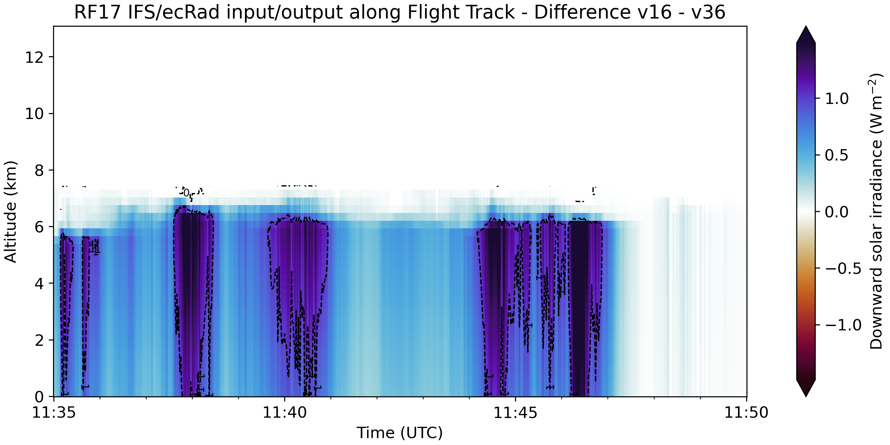
Fig. 32 Difference in short wave downward irradiance along track for RF 17.

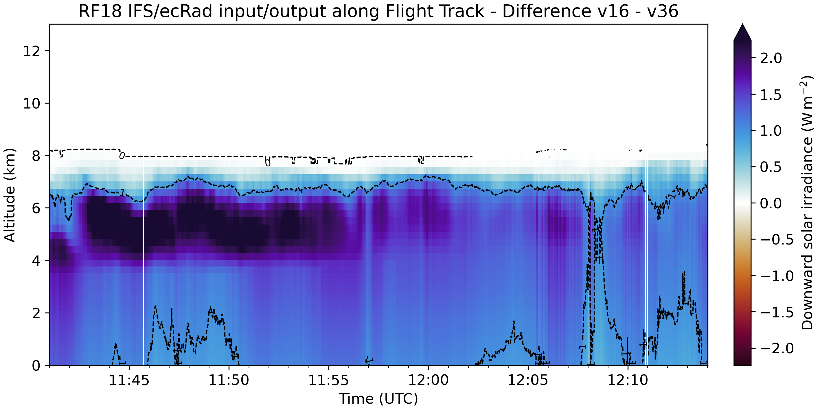
Fig. 33 Difference in short wave downward irradiance along track for RF 18.

As expected the changes only start to appear at cloud top. Another comparison can be done using the upward solar irradiance.

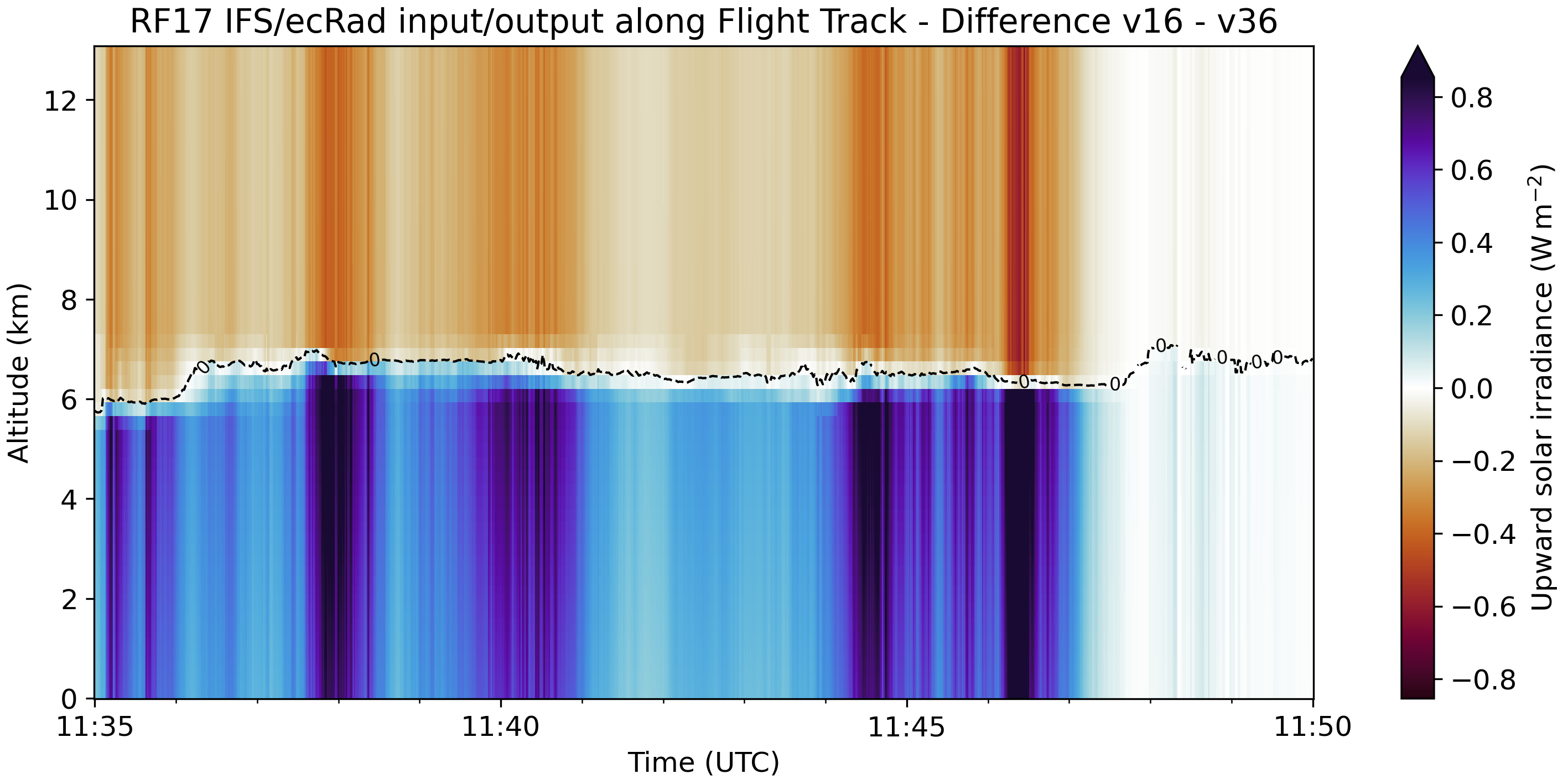
Fig. 34 Difference in short wave upward irradiance along track for RF 17.

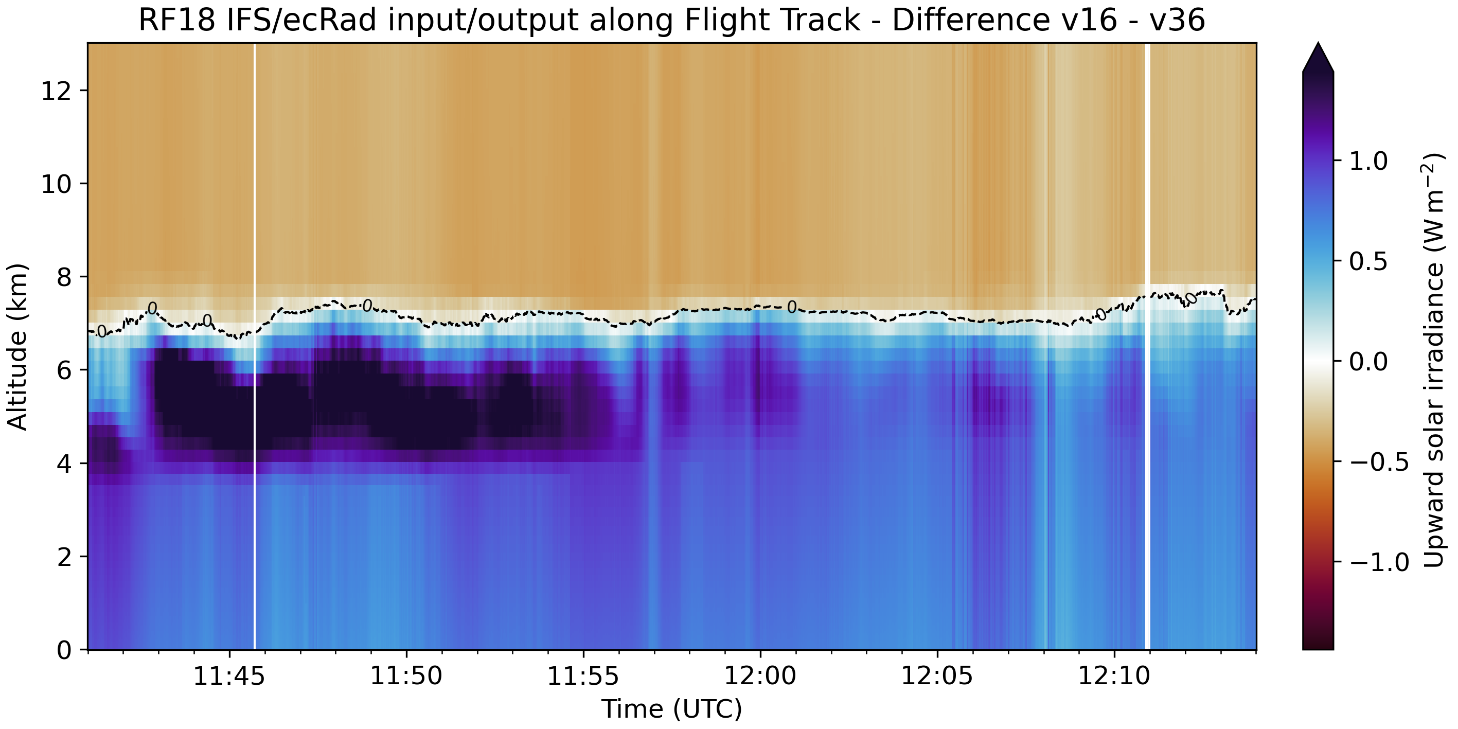
Fig. 35 Difference in short wave upward irradiance along track for RF 18.

We can also take a look on the effect the reduced variability has on the solar transmissivity below cloud.

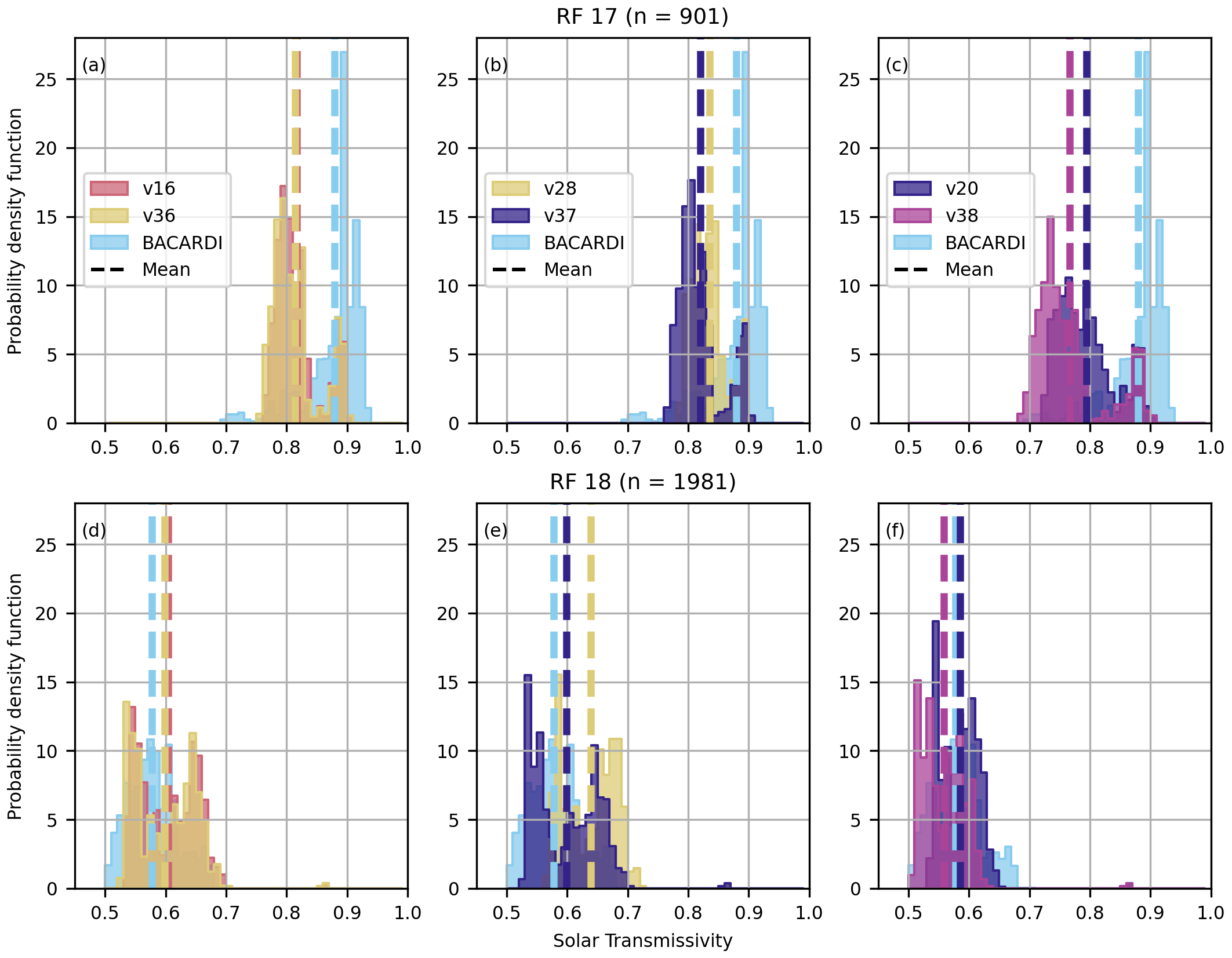
Fig. 36 Solar transmissivity below cloud for RF 17 and RF 18 using the three different ice optic parameterizations Fu-IFS, Yi213 and Baran2016 (from left to right).

Although only minute, a small shift to lower transmissivities can be seen. All in all, the change to a fractional standard deviation of 0 leads to a minor change of the radiative fluxes. Turning the artificially introduced inhomogeneity off, is a better representation of the actual cloud field. Therefore, these new versions are used in the paper and the thesis.

Direct sea ice albdeo

Script: experiments.ecrad_new_direct_sea_ice_albedo.py

author: Johannes Röttenbacher

created: 05.02.2024

Here we investigate the impact the switch to the direct sea ice albedo according to Ebert and Curry [1993] has during the case study section of RF 17. For this we only compare the two reference simulations using the old (v15.1_old_ci_albedo) and the new (v15.1) way of calculating the sw_albedo_direct variable.

At first, we look at the sw_albedo_direct variable used in the simulations and the difference between them.

Fig. 37 Old and new sw_albedo_direct variable and the difference between them.

We can see up to 10% higher values using the new sw_albedo_direct. This also has an impact on the simulated irradiance, which is shown below.

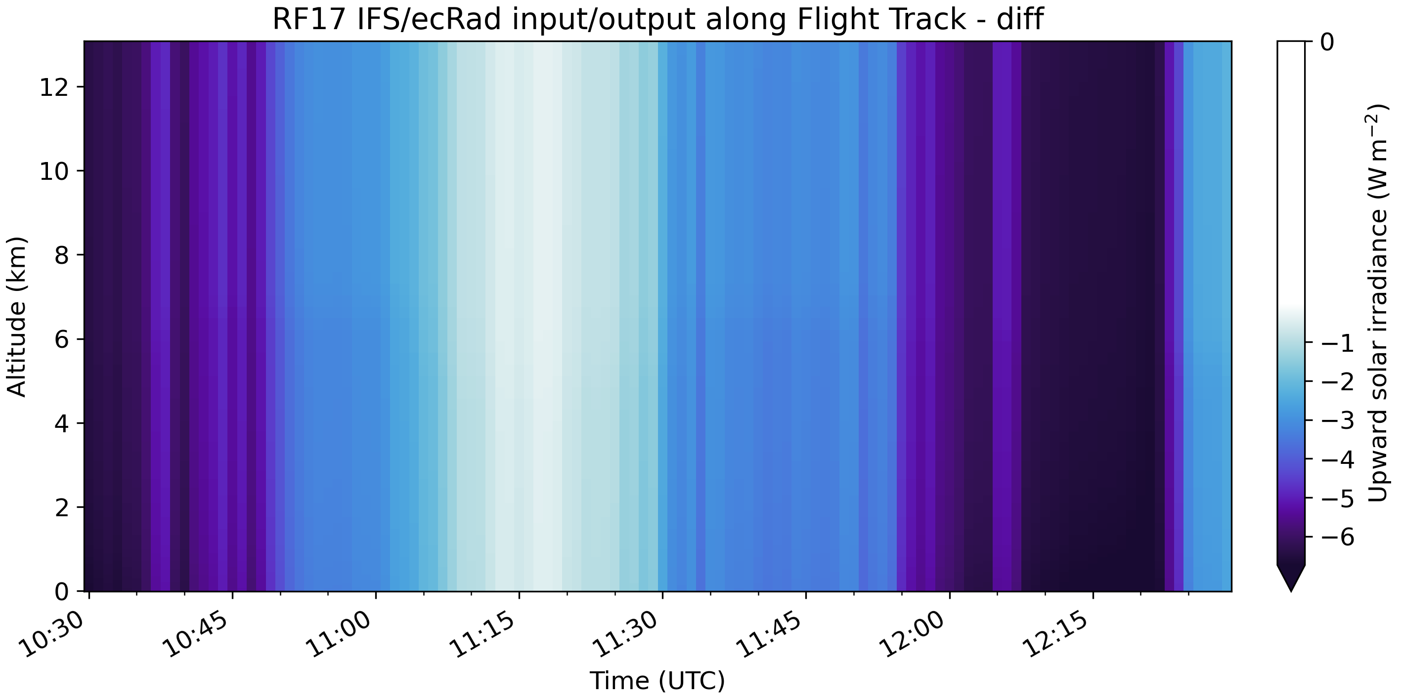
Fig. 38 Difference in solar upward flux between old and new sw_albedo_direct.

The influence on the solar transmissivity, however, is rather small as can be seen when comparing the PDFs of the below cloud values.

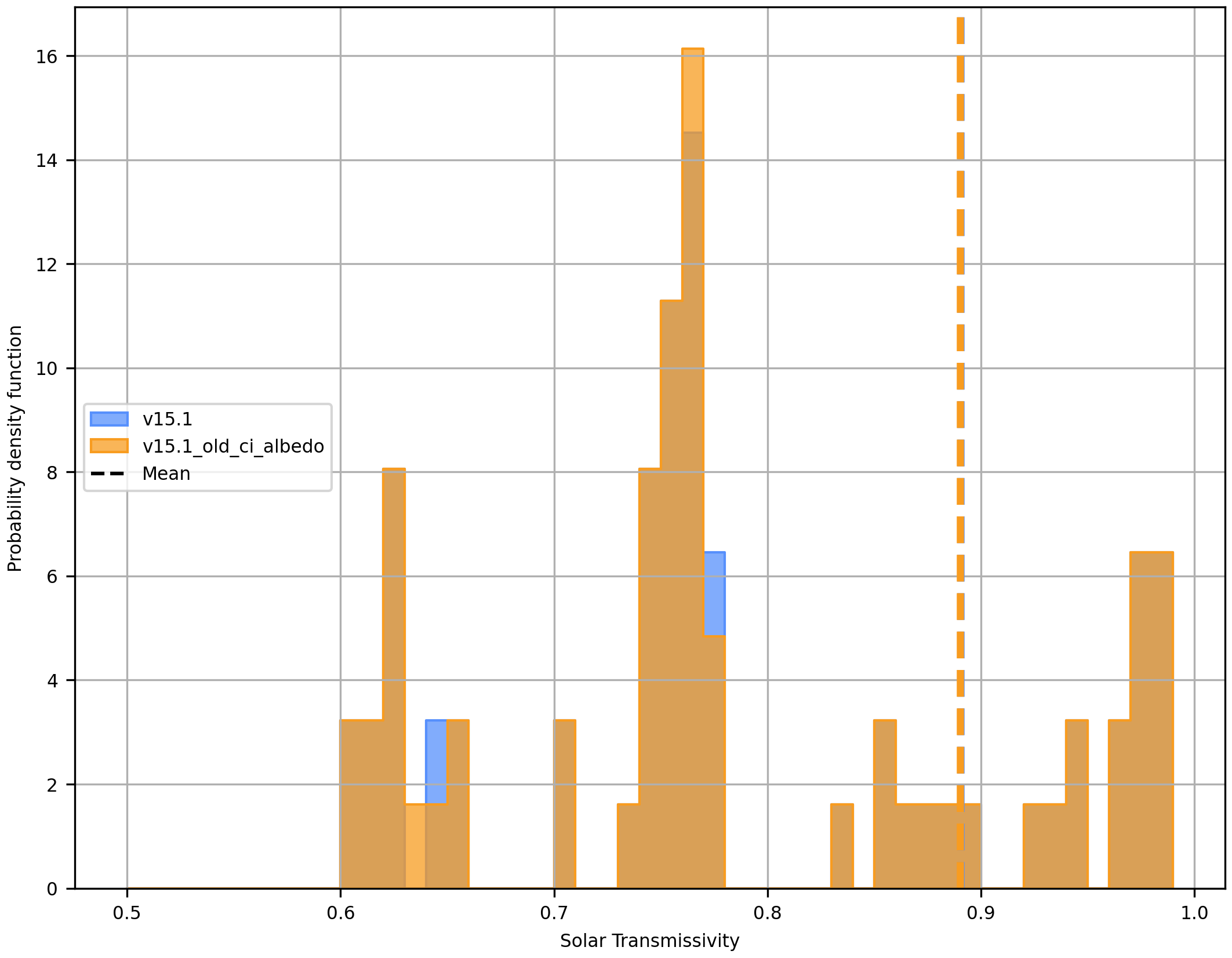
Fig. 39 PDFs of solar transmissivity below cloud for the two cases.

CAMS aerosol climatology

Script: experiments.ecrad_experiment_aerosol.py

3-D effects parameterization

Script: experiments.ecrad_3D_case_study.py

Longwave cloud scattering

Script: experiments.ecrad_lw_cloud_scattering.py

author: Johannes Röttenbacher

created: 27.05.2024

In the ecRad namelist the longwave cloud scattering can be turned off and on (do_lw_cloud_scattering), with on being the default according to the documentation. Here we look at the difference this option makes for the Fu-IFS reference simulation (v15.1). To make sure that this does not affect the short wave calculations, we start with the net short wave flux difference between the new (with lw scattering) and the old simulations.

Fig. 40 Difference in net short wave irradiance between the new (with lw scattering) and the old simulations.

As we can see, there is no difference in the shortwave flux.

We now move on to the difference in longwave downward irradiance.

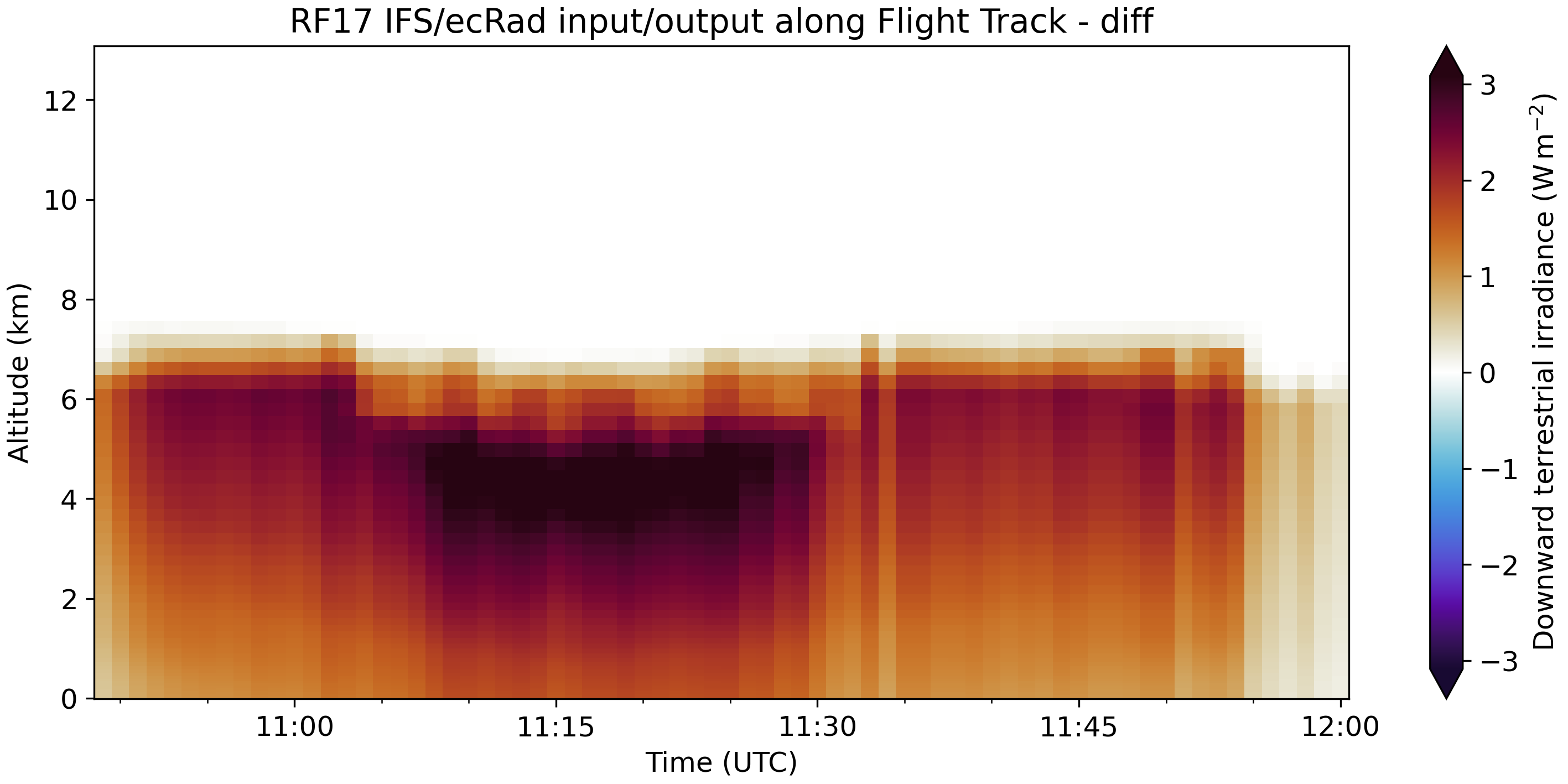
Fig. 41 Difference in longwave downward irradiance along flight track between simulations with longwave cloud scattering and without.

It can be seen that the longwave cloud scattering causes an increased downward irradiance. Thus, more irradiance is scattered by the cloud than absorbed, which is to be expected from this option. The main emitter in the longwave is the surface. Therefore, the longwave upward irradiance should be reduced above the cloud. This can be seen in the next figure.

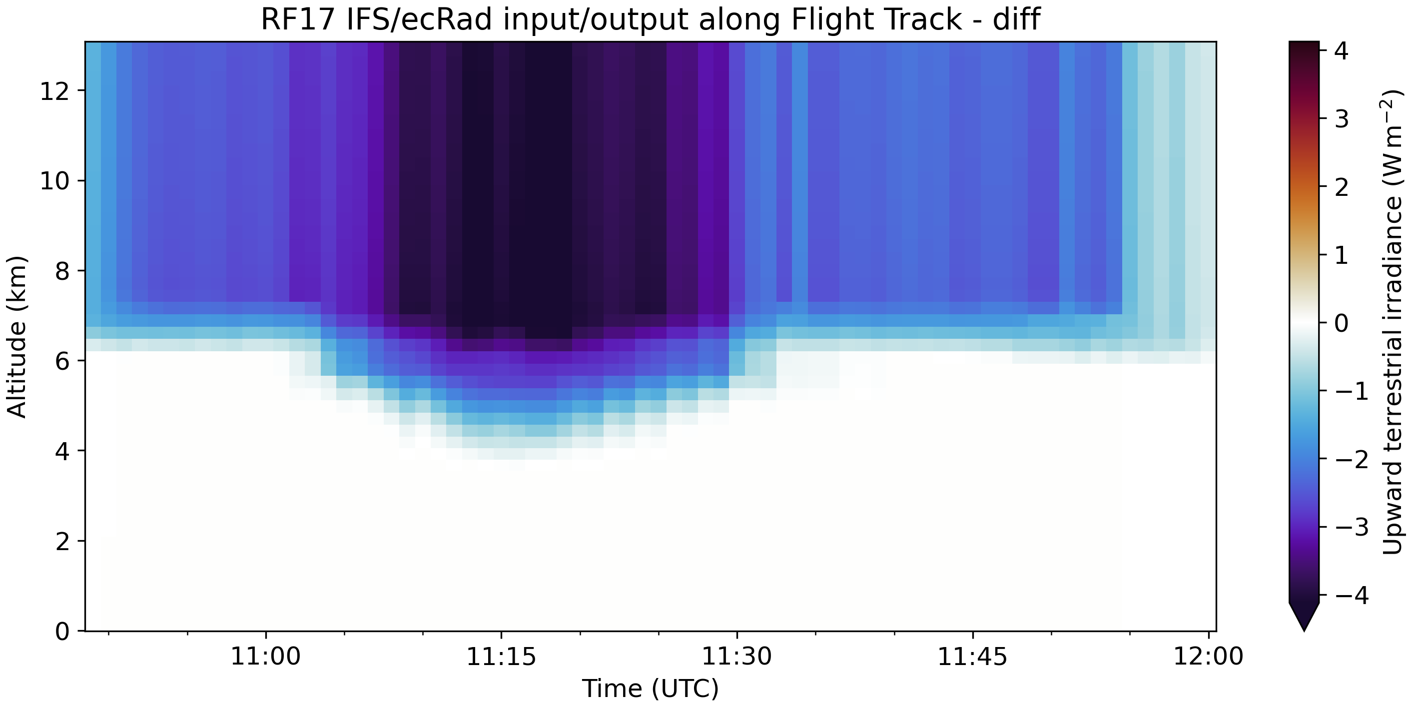
Fig. 42 Difference in longwave upward irradiance along flight track between simulations with longwave cloud scattering and without.

The net longwave flux is generally negative for cirrus cloud scenes. Knowing this the positive difference in net longwave flux shown below means that the net longwave flux with the longwave cloud scattering is less negative. More scattering means less absorption but also less upward irradiance and thus less cooling. Thus, simulations including longwave scattering show less terrestrial cooling for cirrus clouds. As it is the default option, longwave cloud scattering will be turned on in all simulations.

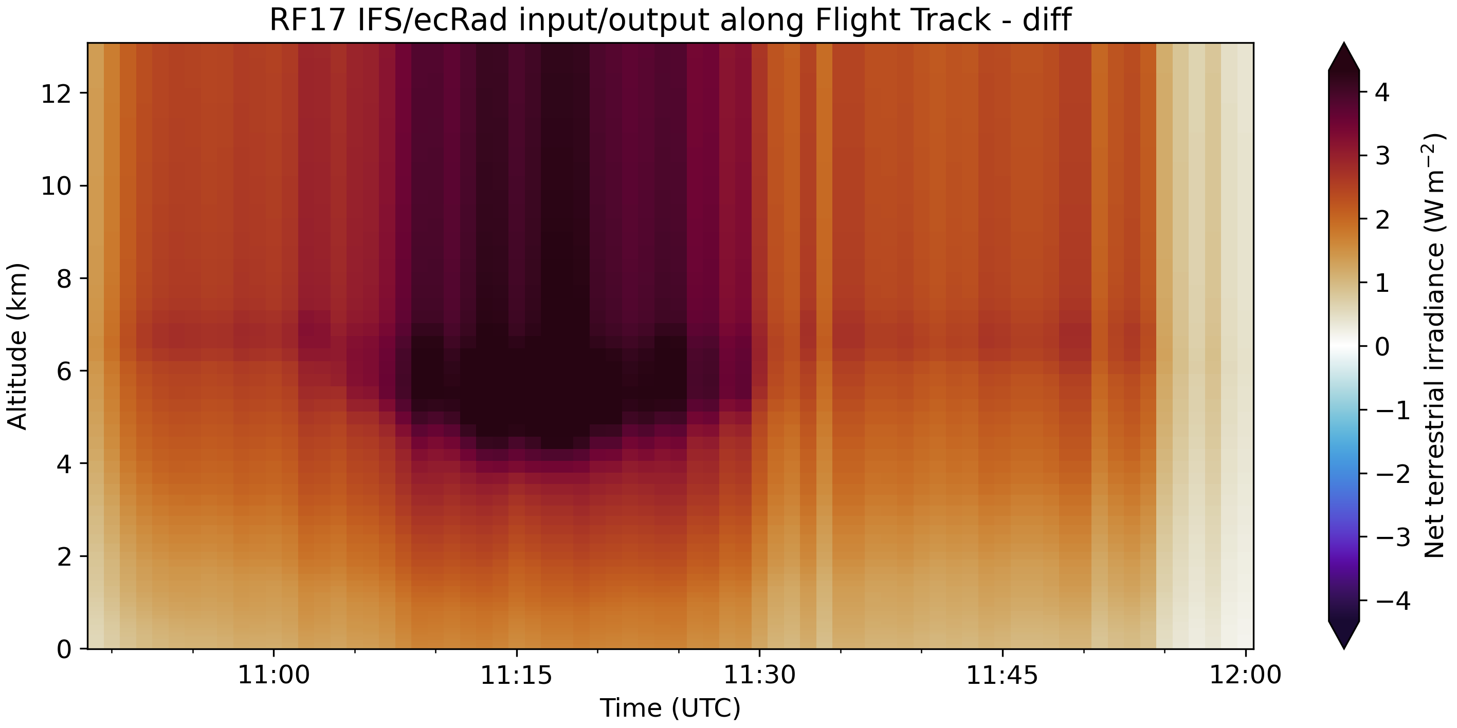
Fig. 43 Difference in net longwave irradiance along flight track between simulations with longwave cloud scattering and without.

Humidity from dropsondes

Script: experiments.ecrad_humidity_from_dropsonde.py

ecRad Setups

Setup ala Hanno

• manually enter decorrelation length in namelist depending on latitude (output from ecrad_read_ifs.py)

• solar constant: distance sun-earth from heavens above website, calculate solar constant in Excel ({campaign}_solar_constant.xlsx)

• use ozone data from ozone sondes → http://www.ndaccdemo.org/

Standard IFS setup for HALO-(AC)³

• namelists: IFS_namelist_jr_20220411_v15.nam, …

• manually entered mean decorrelation length for case study region

• solar constant given

• ozone data from trace gas climatology

• aerosol disabled

libRadtran Setups and Experiments

HALO-(AC)³ BACARDI broadband simulation for BACARDI nc file

• use Longyearbyen radiosonde for vertical profile of relative humidity

• surface temperature → unclear, ask Anna

  • set to 293.15K in script but might have been different for Anna’s simulation

• for details see: processing.libradtran_write_input_file_bacardi.py

• filename: HALO-AC3_HALO_libRadtran_bb_clearsky_simulation_[solar/terrestrial]_[yyyymmdd]_RF[xx].nc

HALO-(AC)³ BACARDI below cloud RF17

Script: experiments.libradtran_write_input_file_below_cloud.py Folder: exp0

Simulate a clearsky situation above/below the cirrus while HALO was below/above it. This can be used to compare the above and below cloud simulation at the same time to derive the atmospheric absorption. Using this the actual influence of the cirrus can be derived.

• use dropsonde profiles as input

• use the IFS sea ice albedo parameterization (TODO)

HALO-(AC)³ BACARDI/SMART clear sky simulation with sea ice

Scripts:

• experiments.libradtran_write_input_file_seaice.py

• experiments.libradtran_run_uvspec_seaice.py

Folders:

• seaice_smart: The first run of this experiment was done for the wavelength range 250 - 2225 nm on accident

• seaice_solar, seaice_thermal

Set up libRadtran for clearsky simulation along flight path for BACARDI with sea ice albedo included

Input:

• Dropsonde profiles from the flight

• sea ice albedo parameterization from the IFS

• sea ice concentration from IFS

Required User Input:

• campaign

• flight_key (e.g. ‘RF17’)

• time_step (e.g. ‘minutes=1’)

• use_smart_ins flag

• solar_flag

• integrate flag

• input_path, this is where the files will be saved to be executed by uvspec

Output:

• log file

• input files for libRadtran simulation along flight track

The idea for this script is to generate a dictionary with all options that should be set in the input file. New options can be manually added to the dictionary. The options are linked to the page in the manual where they are described in more detail. Set options to “None” if you don’t want to use them.

Furthermore, an albedo file is generated for the solar simulation using the sea ice albedo parameterization from Ebert and Curry [1993] and the open ocean albedo parameterization from Taylor et al. [1996]. To allow simulations in the thermal infrared region an additional albedo band between 2501 and 4400 nm is added. The sea ice albedo is set to 0 in this band.

For the terrestrial simulation the albedo is set to a constant value depending on surface type over all wavelengths.

The atmosphere is provided by the closest dropsonde measurement from HALO which was converted to the right input format by an IDL script.

author: Johannes Röttenbacher

HALO-(AC)³ BACARDI/SMART clear sky simulation with sea ice up to 5000nm

Scripts:

• experiments.libradtran_write_input_file_seaice_2.py

• experiments.libradtran_run_uvspec_seaice.py

Folders:

• seaice_2_solar

Notes:

The same execution script is used as for the previous sea ice experiment. Only libradtran_dir in line 40 and nc_filepath in line 208 are adjusted.

Set up libRadtran for clearsky simulation along flight path for BACARDI with sea ice albedo included up to 5000nm

Input:

• Dropsonde profiles from the flight

• sea ice albedo parameterization from the IFS

• sea ice concentration from IFS

Required User Input:

• campaign

• flight_key (e.g. ‘RF17’)

• time_step (e.g. ‘minutes=1’)

• use_smart_ins flag

• solar_flag

• integrate flag

• input_path, this is where the files will be saved to be executed by uvspec

Output:

• log file

• input files for libRadtran simulation along flight track

The idea for this script is to generate a dictionary with all options that should be set in the input file. New options can be manually added to the dictionary. The options are linked to the page in the manual where they are described in more detail. Set options to “None” if you don’t want to use them.

Furthermore, an albedo file is generated for the solar simulation using the sea ice albedo parameterization from Ebert and Curry [1993] and the open ocean albedo parameterization from Taylor et al. [1996]. To allow simulations in the thermal infrared region an additional albedo band between 2501 and 4500 nm is added. The sea ice albedo is set to 0 in this band.

For the terrestrial simulation the albedo is set to a constant value depending on surface type over all wavelengths.

The atmosphere is provided by a dropsonde measurement which was converted to the right input format by an IDL script.

author: Johannes Röttenbacher

HALO-(AC)³ Icecloud over sea ice experiment

Name: iceloud

Scripts:

• experiments.libradtran_write_input_file_icecloud.py

• experiments.libradtran_run_uvspec_experiment.py

• experiments.libradtran_icecloud_sensitivity_study.py

Folders:

• icecloud

Icecloud Setup

author: Johannes Röttenbacher

created: 22-02-2023

Set up libRadtran like ecRad using input from the IFS and defining an ice cloud for a sensitivity study

Input:

• IFS processed input file from ecrad_read_ifs.py

Required User Input:

• campaign

• flight_key (e.g. ‘RF17’)

• time_step (e.g. ‘minutes=1’)

• use_smart_ins flag

• integrate flag

• input_path, this is where the files will be saved to be executed by uvspec

• different iwc and re_ice values

Output:

• log file

• input files for libRadtran simulation along flight track

The idea for this script is to generate a dictionary with all options that should be set in the input file. New options can be manually added to the dictionary. The options are linked to the page in the manual where they are described in more detail. Set options to “None” if you don’t want to use them.

Furthermore, an atmosphere, an albedo and an ice cloud file are generated.

Variables to add to the atmosphere files:

1 Altitude above sea level in km → IFS 2 Pressure in hPa → IFS 3 Temperature in K → IFS 4 air density in cm−3 → IFS 5 Ozone density in cm−3 → sonde (CAMS) 6 Oxygen density in cm−3 → constant 7 Water vapour density in cm−3 → IFS 8 CO2 density in cm−3 → constant (CAMS)

Variables to add to the albedo files:

• spectral albedo from IFS

Variables to add to the cloud files:

• cloud fraction (cloud fraction file)

• ice water content, ice effective radius (ice cloud file)

author: Johannes Röttenbacher

created: 01.03.2023

Results of icecloud sensitivity simulations with libRadtran

HALO-(AC)³ Icecloud along flight track for RF17

Name: icecloud2

Scripts:

• experiments.libradtran_write_input_file_icecloud2.py

• experiments.libradtran_run_uvspec_experiment.py

Folders:

• icelcoud2

Icecloud 2 Setup

author: Johannes Röttenbacher

created: 03-03-2023

Set up libRadtran like ecRad using input from the IFS and defining an ice cloud along track for a sensitivity study

Simulate an ice cloud along the case study period of RF17 (2022-04-11 10:30 - 12:30 UTC) with different IWC and \(r_{eff, ice}\) at 6.5 to 7.5 km altitude. Generate output at every 100m in the vertical.

Input:

• IFS processed input file from ecrad_read_ifs.py

Required User Input:

• campaign

• flight_key (e.g. ‘RF17’)

• time_step (e.g. ‘minutes=1’)

• use_smart_ins flag

• integrate flag

• input_path, this is where the files will be saved to be executed by uvspec

• different iwc and re_ice values

Output:

• log file

• input files for libRadtran simulation along flight track

The idea for this script is to generate a dictionary with all options that should be set in the input file. New options can be manually added to the dictionary. The options are linked to the page in the manual where they are described in more detail. Set options to “None” if you don’t want to use them.

Furthermore, an atmosphere, an albedo and an ice cloud file are generated.

Variables to add to the atmosphere files:

1 Altitude above sea level in km → IFS 2 Pressure in hPa → IFS 3 Temperature in K → IFS 4 air density in cm−3 → IFS 5 Ozone density in cm−3 → sonde (CAMS) 6 Oxygen density in cm−3 → constant 7 Water vapour density in cm−3 → IFS 8 CO2 density in cm−3 → constant (CAMS)

Variables to add to the albedo files:

• spectral albedo from IFS

Variables to add to the cloud files:

• cloud fraction (cloud fraction file)

• ice water content, ice effective radius (ice cloud file)

HALO-(AC)³ Varcloud simulation above cloud

Name: varcloud

Scripts:

• experiments.libradtran_write_input_file_varcloud.py

• experiments.libradtran_run_uvspec_experiment.py

Folders:

• varcloud

Varcloud Setup

author: Johannes Röttenbacher

created: 28-03-2023

Set up libRadtran like ecRad using input from the IFS and defining an ice cloud along track using the VarCloud output from Florian Ewald, LMU.

Simulate an ice cloud along the above cloud section RF17 (2022-04-11 10:48:47 - 11:07:14 UTC) with IWC and \(r_{eff, ice}\) from the VarCloud retrieval. Generate output at every height level defined by the VarCloud input.

Input:

• IFS processed input file from ecrad_read_ifs.py

• VarCloud output file provided by Florian Ewald

Required User Input:

• campaign

• flight_key (e.g. ‘RF17’)

• time_step (e.g. ‘minutes=1’)

• use_smart_ins flag

• integrate flag

• input_path, this is where the files will be saved to be executed by uvspec

Output:

• log file

• input files for libRadtran simulation along flight track

The idea for this script is to generate a dictionary with all options that should be set in the input file. New options can be manually added to the dictionary. The options are linked to the page in the manual where they are described in more detail. Set options to “None” if you don’t want to use them.

Furthermore, an atmosphere, an albedo and an ice cloud file are generated.

Variables to add to the atmosphere files:

1 Altitude above sea level in km → IFS 2 Pressure in hPa → IFS 3 Temperature in K → IFS 4 air density in cm−3 → IFS 5 Ozone density in cm−3 → sonde (CAMS) 6 Oxygen density in cm−3 → constant 7 Water vapour density in cm−3 → IFS 8 CO2 density in cm−3 → constant (CAMS)

Variables to add to the albedo files:

• spectral albedo from IFS

Variables to add to the cloud files:

• cloud fraction (cloud fraction file)

• ice water content, ice effective radius (ice cloud file)